An analysis of the algebraic structures in the context of intertemporal choice

Salvador Cruz Rambaud; Blas Torrecillas Jover; Salvador Cruz Rambaud; Blas Torrecillas Jover

doi:10.3934/math.2022575

AIMS Mathematics

2022, Volume 7, Issue 6: 10315-10343. doi: 10.3934/math.2022575

Previous Article Next Article

Research article

An analysis of the algebraic structures in the context of intertemporal choice

Salvador Cruz Rambaud ^{1
,
,},
Blas Torrecillas Jover ²

1.
Departamento de Economía y Empresa. Universidad de Almería, La Cañada de San Urbano, s/n, 04120, Almería, Spain
2.
Departamento de Matemáticas. Universidad de Almería, La Cañada de San Urbano, s/n, 04120, Almería, Spain

Received: 19 November 2021 Revised: 07 February 2022 Accepted: 01 March 2021 Published: 24 March 2022
MSC : 91G99

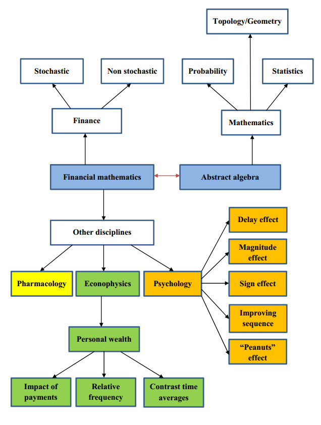
Framework and justification: The content of this paper is located on the intersection of two fields: Finance and Algebra. In effect, the current dynamism shown by most financial instruments makes it necessary to endow the foundations of finance with, as general as possible, algebraic structures. Therefore, the objective of this paper is to provide a novel view of the fundamentals of finance by using purely algebraic concepts and structures, more specifically the properties of separability and additivity of the involved discount functions and their corresponding operators. This approach provides more flexibility to the axioms of financial mathematics, so anticipating potential changes in the behavior of the so-called "rational" decision makers. Methodologically, this paper uses a variety of algebraic tools which fit the intuition behind the financial logic. Indeed, the main contribution of the paper is the wide variety of algebraic concepts belonging to the abstract algebra which can be applied to describe the behavior of intertemporal choices.
- intertemporal choice,
- discount function,
- additivity,
- vector space,
- affine space,
- quiver
Citation: Salvador Cruz Rambaud, Blas Torrecillas Jover. An analysis of the algebraic structures in the context of intertemporal choice[J]. AIMS Mathematics, 2022, 7(6): 10315-10343. doi: 10.3934/math.2022575

Related Papers:

Abstract

Framework and justification: The content of this paper is located on the intersection of two fields: Finance and Algebra. In effect, the current dynamism shown by most financial instruments makes it necessary to endow the foundations of finance with, as general as possible, algebraic structures. Therefore, the objective of this paper is to provide a novel view of the fundamentals of finance by using purely algebraic concepts and structures, more specifically the properties of separability and additivity of the involved discount functions and their corresponding operators. This approach provides more flexibility to the axioms of financial mathematics, so anticipating potential changes in the behavior of the so-called "rational" decision makers. Methodologically, this paper uses a variety of algebraic tools which fit the intuition behind the financial logic. Indeed, the main contribution of the paper is the wide variety of algebraic concepts belonging to the abstract algebra which can be applied to describe the behavior of intertemporal choices.

References

[1]	J. Aczél, Lectures on functional equations and their applications (Mathematics in Science and Engineering, Volume 19), New York: Academic Press, 1966.
[2]	A. Adamou, Y. Berman, D. Mavroyiannis, O. Peters, Microfoundations of discounting, Decis. Anal., 18 (2021), 257–272. https://doi.org/10.1287/deca.2021.0436 doi: 10.1287/deca.2021.0436
[3]	D. O. Cajueiro, A note on the relevance of the $q$-exponential function in the context of intertemporal choices, Physica A, 364 (2006), 385–388. https://doi.org/10.1016/j.physa.2005.08.056 doi: 10.1016/j.physa.2005.08.056
[4]	A. H. Clifford, G. B. Preston, The Algebraic Theory of Semigroups, Providence, RI: Amer. Math. Soc., 1961. https://doi.org/10.1090/surv/007.1
[5]	S. Cruz Rambaud, Some new ideas in the concept of financial law, Decis. Econ. Financ., 20 (1997), 23–43. https://doi.org/10.1007/BF02688987 doi: 10.1007/BF02688987
[6]	S. Cruz Rambaud, J. García Pérez, The accounting system as an algebraic automaton, Int. J. Intell. Syst., 20 (2005), 827–842. https://doi.org/10.1002/int.20095 doi: 10.1002/int.20095
[7]	S. Cruz Rambaud, J. García Pérez, R. A. Nehmer, D. J. S. Robinson, Algebraic Models For Accounting Systems, Singapore: World Scientific, 2010.
[8]	S. Cruz Rambaud, I. González Fernández, V. Ventre, Modeling the inconsistency in intertemporal choice: The generalized Weibull discount function and its extension, Ann. Financ., 14 (2018), 415–426. https://doi.org/10.1007/s10436-018-0318-3 doi: 10.1007/s10436-018-0318-3
[9]	S. Cruz Rambaud, J. López Pascual, M. Á. del Pino Álvarez, Preferences over sequences of payments: A new validation of the $q$-exponential discounting, Physica A, 515 (2019), 332–345. https://doi.org/10.1016/j.physa.2018.09.169 doi: 10.1016/j.physa.2018.09.169
[10]	S. Cruz Rambaud, M. J. Muñoz Torrecillas, A generalization of the $q$-exponential discounting function, Physica A, 392 (2013), 3045–3050. https://doi.org/10.1016/j.physa.2013.03.009 doi: 10.1016/j.physa.2013.03.009
[11]	S. Cruz Rambaud, M. J. Muñoz Torrecillas, Measuring impatience in intertemporal choice, PLoS ONE, 11 (2016), e0149256. https://doi.org/10.1371/journal.pone.0149256 doi: 10.1371/journal.pone.0149256
[12]	S. Cruz Rambaud, M. J. Muñoz Torrecillas, T. Takahashi, Observed and normative discount functions in addiction and other diseases, Front. Pharmacol., 8 (2017), article 416. https://doi.org/10.3389/fphar.2017.00416 doi: 10.3389/fphar.2017.00416
[13]	S. Cruz Rambaud, M. J. Muñoz Torrecillas, A. Garcia, A mathematical analysis of the improving sequence effect for monetary rewards, Front. Appl. Math. Stat., 4 (2018), article 55. https://doi.org/10.3389/fams.2018.00055 doi: 10.3389/fams.2018.00055
[14]	S. Cruz Rambaud, P. Ortiz Fernández, Delay effect and subadditivity. Proposal of a new discount function: The asymmetric exponential discounting, Mathematics, 8 (2020), 367. https://doi.org/10.3390/math8030367 doi: 10.3390/math8030367
[15]	S. Cruz Rambaud, I. M. Parra Oller, M. C. Valls Martínez, The amount-based deformation of the $q$-exponential discount function: A joint analysis of delay and magnitude effects, Physica A, 508 (2018), 788–796. https://doi.org/10.1016/j.physa.2018.05.152 doi: 10.1016/j.physa.2018.05.152
[16]	S. Cruz Rambaud, A. M. Sánchez Pérez, The magnitude and "peanuts" effects: Searching implications, Front. Appl. Math. Stat., 4 (2018), article 36. https://doi.org/10.3389/fams.2018.00036 doi: 10.3389/fams.2018.00036
[17]	S. Cruz Rambaud, B. Torrecillas Jover, An extension of the concept of derivative: Its application to intertemporal choice, Mathematics, 8 (2020), 696. https://doi.org/10.3390/math8050696 doi: 10.3390/math8050696
[18]	S. Cruz Rambaud, V. Ventre, Deforming time in a non-additive discount function, Int. J. Intell. Syst., 32 (2017), 467–480. https://doi.org/10.1002/int.21842 doi: 10.1002/int.21842
[19]	J. C. Do Nascimento, The personal wealth importance to the intertemporal choice, Physica A, 565 (2021), 125559. https://doi.org/10.1016/j.physa.2020.125559 doi: 10.1016/j.physa.2020.125559
[20]	A. Garcia, M. J. Muñoz Torrecillas, S. Cruz Rambaud, The improving sequence effect on monetary sequences, Heliyon, 6 (2020), e05643. https://doi.org/10.1016/j.heliyon.2020.e05643 doi: 10.1016/j.heliyon.2020.e05643
[21]	M. Kilp, U. Knauer, A. V. Mikhalev, Monoids, Acts and Categories with Applications to Wreath Products and Graphs, Volume 29 of Expositions in Mathematics, Berlin: Walter de Gruyter, 2000. https://doi.org/10.1515/9783110812909
[22]	J. M. Howie, An Introduction to Semigroup Theory, New York: Academic Press, 1976.
[23]	J. Lambek, P. J. Scott, Introduction to Higher Order Categorical Logic, Cambridge: Cambridge Univ. Press, 1986.
[24]	Z. Liu, R. Gao, C. Zhou, N. Ma, Two-period pricing and strategy choice for a supply chain with dual uncertain information under different profit risk levels, Comput. In. Eng., 136 (2019), 173–186. https://doi.org/10.1016/j.cie.2019.07.029 doi: 10.1016/j.cie.2019.07.029
[25]	N. I. Mahmudov, M. E. Keleshteri, On a class of generalized $q$-Bernoulli and $q$-Euler polynomials, Adv. Differ. Equ-Ny., 115 (2013), 1–10.
[26]	G. Maze, C. Monico, J. Rosenthal, Public key criptography based in semigroup actions, Adv. Math. Commun., 1 (2007), 489–507. https://doi.org/10.3934/amc.2007.1.489 doi: 10.3934/amc.2007.1.489
[27]	R. A. Nehmer, Accounting systems as first order axiomatic models: Consequences for information theory, Int. J. Math. Oper. Res., 2 (2010), 99–112. https://doi.org/10.1504/IJMOR.2010.029692 doi: 10.1504/IJMOR.2010.029692
[28]	R.A. Nehmer, D.J.S. Robinson, An algebraic model for the representation of accounting systems, Ann. Oper. Res., 71 (1997), 179–198. https://doi.org/10.1023/A:1018915430594 doi: 10.1023/A:1018915430594
[29]	O. Peters, The ergodicity problem in economics, Nature Physics, 15 (2019), 1216–1221. https://doi.org/10.1038/s41567-019-0732-0 doi: 10.1038/s41567-019-0732-0
[30]	O. Peters, A. Adamou, The time interpretation of expected utility theory, arXiv: 1801.03680, (2018).
[31]	O. Peters, M. Gell-Mann, Evaluating gambles using dynamics, Chaos: An Interdisciplinary Journal of Nonlinear Science, 26 (2016), 023103. https://doi.org/10.1063/1.4940236 doi: 10.1063/1.4940236
[32]	K. I. M. Rohde, Measuring decreasing and increasing impatience, Manag. Sci., 65 (2019), 1700–1716. https://doi.org/10.1287/mnsc.2017.3015 doi: 10.1287/mnsc.2017.3015
[33]	S. S. Stevens, On the psycho physical law, Psychol. Rev., 64 (1957), 153–181. https://doi.org/10.1037/h0046162 doi: 10.1037/h0046162
[34]	F. Sun, X. Wei, Pension discount rate and investor sentiment, Manag. Financ., 45 (2019), 781–792.
[35]	T. Takahashi, Loss of self-control in intertemporal choice may be attributable to logarithmic time-perception, Med. Hypotheses, 65 (2005), 691–693. https://doi.org/10.1016/j.mehy.2005.04.040 doi: 10.1016/j.mehy.2005.04.040
[36]	K. Takeuchi, Non-parametric test of time consistency: Present bias and future bias, Games Econ. Behav., 71 (2011), 456–478. https://doi.org/10.1016/j.geb.2010.05.005 doi: 10.1016/j.geb.2010.05.005
[37]	G. J. Tellis, F. S. Zufryden, Tackling the retailer decision maze: Which brands to discount, how much, when and why?, Market. Sci., 14 (1995), 271–299. https://doi.org/10.1287/mksc.14.3.271 doi: 10.1287/mksc.14.3.271
[38]	B. Torrecillas Jover, S. Cruz Rambaud, Las leyes financieras a través de los factores, Cuadernos Aragoneses de Economía, 5 (1995), 459–473.
[39]	C. Tsallis, What are the numbers that experiments provide?, Quim. Nova, 17 (1994), 468–471.

Reader Comments

Your name:*

Email:*
© 2022 the Author(s), licensee AIMS Press. This is an open access article distributed under the terms of the Creative Commons Attribution License (http://creativecommons.org/licenses/by/4.0)