As is well known, the utility function is significant for solving the real-time pricing problem of smart grids. Based on a new utility function, the social welfare maximization model is considered in this paper. First, we transform the social welfare maximization model into a smooth system of equations using Krush-Kuhn-Tucker (KKT) conditions, then propose a two-step smoothing Levenberg-Marquardt method with global convergence, where an LM step and an approximate LM step are computed at every iteration. The local convergence of the algorithm is cubic under the local error bound condition, which is weaker than the nonsingularity. The simulation results show that, the algorithm can not only reduce the user's electricity consumption but also improve the total social welfare at the most time when compared with the fixed pricing method. Additionally, when different values of the approximating parameter are adopted in a smoothing quasi-Newton method, the price tends to that obtained by the present algorithm. Furthermore, the CPU time of the one-step smoothing Levenberg-Marquardt algorithm and the proposed algorithm are also listed.
Citation: Linsen Song, Gaoli Sheng. A two-step smoothing Levenberg-Marquardt algorithm for real-time pricing in smart grid[J]. AIMS Mathematics, 2024, 9(2): 4762-4780. doi: 10.3934/math.2024230
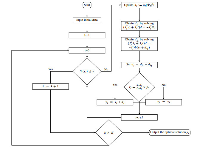
As is well known, the utility function is significant for solving the real-time pricing problem of smart grids. Based on a new utility function, the social welfare maximization model is considered in this paper. First, we transform the social welfare maximization model into a smooth system of equations using Krush-Kuhn-Tucker (KKT) conditions, then propose a two-step smoothing Levenberg-Marquardt method with global convergence, where an LM step and an approximate LM step are computed at every iteration. The local convergence of the algorithm is cubic under the local error bound condition, which is weaker than the nonsingularity. The simulation results show that, the algorithm can not only reduce the user's electricity consumption but also improve the total social welfare at the most time when compared with the fixed pricing method. Additionally, when different values of the approximating parameter are adopted in a smoothing quasi-Newton method, the price tends to that obtained by the present algorithm. Furthermore, the CPU time of the one-step smoothing Levenberg-Marquardt algorithm and the proposed algorithm are also listed.

| [1] |
C. Dang, X. F. Wang, C. C. Shao, X. L. Wang, Distributed generation planning for diversified participants in demand response to promote renewable energy integration, J. Mod. Power Syst. Cle., 7 (2019), 1559–1572. https://doi.org/10.1007/s40565-019-0506-9 doi: 10.1007/s40565-019-0506-9

|
| [2] |
J. Lin, B. Xiao, H. Zhang, X. Y. Yang, P. Zhao, A novel multitype-users welfare equilibrium based real-time pricing in smart grid, Future Gener. Comp. Sy., 108 (2020), 145–160. https://doi.org/10.1016/j.future.2020.02.013 doi: 10.1016/j.future.2020.02.013
|
| [3] |
R. Rotas, M. Fotopoulou, P. Drosatos, D. Rakopoulos, N. Nikolopoulos, Adaptive dynamic building envelopes with solar power components: Annual performance assessment for two pilot sites, Energies, 16 (2023). https://doi.org/10.3390/en16052148 doi: 10.3390/en16052148
|
| [4] |
R. Mohamed, A. Mohammad, Optimal planning and operation of grid-connected PV/CHP/battery energy system considering demand response and electric vehicles for a multi-residential complex building, J. Energy. Stor., 72 (2023), 108198. https://doi.org/10.1016/j.est.2023.108198 doi: 10.1016/j.est.2023.108198
|
| [5] |
E. Bellos, P. Lykas, C. Tzivanidis, Performance analysis of a zero-energy building using photovoltaics and hydrogen storage, Appl. Syst. Innov., 6 (2023), 43. https://doi.org/10.3390/asi6020043 doi: 10.3390/asi6020043
|
| [6] |
S. Nojavan, K. Zare, Optimal energy pricing for consumers by electricity retailer, Int. J. Elec. Power, 102 (2018), 401–412. https://doi.org/10.1016/j.ijepes.2018.05.013 doi: 10.1016/j.ijepes.2018.05.013
|
| [7] |
Z. Wang, R. Paranjape, Z. Chen, K. Zeng, Layered stochastic approach for residential demand response based on real-time pricing and incentive mechanism, IET Gener. Transm. Dis., 14 (2020), 349–524. https://doi.org/10.1049/iet-gtd.2019.1135 doi: 10.1049/iet-gtd.2019.1135
|
| [8] |
L. Tao, Y. Gao, Real-time pricing for smart grid with distributed energyand storage: A noncooperative game method considering spatially and temporally coupled constraints, Int. J. Elec. Power, 115 (2020), 105487. https://doi.org/10.1016/j.ijepes.2019.105487 doi: 10.1016/j.ijepes.2019.105487
|
| [9] |
Y. M. Dai, Y. Q. Yang, M. M. Leng, A Novel alternative energy trading mechanism for different users considering value-added service and price competition, Comput. Ind. Eng., 172 (2022), 108531. https://doi.org/10.1016/j.cie.2022.108531 doi: 10.1016/j.cie.2022.108531
|
| [10] |
S. Nojavan, K. Zare, B. Mohammadi-Ivatloo, Risk-based framework for supplying electricity from renewable generation-owning retailers to price-sensitive customers using information gap decision theory, Inter. J. Elec. Power, 93 (2017), 156–170. https://doi.org/10.1016/j.ijepes.2017.05.023 doi: 10.1016/j.ijepes.2017.05.023
|
| [11] |
W. Zhang, J. Li, G. Chen, Z. Y. Dong, K. P. Wong, A comprehensive model with fast solver for optimal energy scheduling in RTP environment, IEEE T. Smart Grid., 8 (2017), 2314–2323. https://doi.org/10.1109/TSG.2016.2522947 doi: 10.1109/TSG.2016.2522947
|
| [12] |
H. B. Zhu, Y. Gao, Y. Hou, T. Li, Real-time pricing considering different type of users based on Markov decision processes in smart grid, Syst. Eng.-Theor. Pract., 38 (2018), 807–816. https://doi.org/10.12011/1000-6788(2018)03-0807-10 doi: 10.12011/1000-6788(2018)03-0807-10
|
| [13] |
H. J. Wang, Y. Gao, Research on the real-time pricing of smart grid based on nonsmooth equations, J. Syst. Eng., 33 (2018), 34–41. https://doi.org/10.13383/j.cnki.jse.2018.03.004 doi: 10.13383/j.cnki.jse.2018.03.004
|
| [14] | Y. Y. Li, J. X. Li, Y. Z. Dang, Smoothing Newton algorithm for real-time pricing of smart grid based on KKT conditions, J. Sys. Sci. Math. Sci., 40 (2020), 646–656. |
| [15] |
Y. Y. Li, J. X. Li, J. J. He, S. Y. Zhang, The real-time pricing optimization model of smart grid on the utility function of the logistic function, Energy, 224 (2021), https://doi.org/10.1016/j.energy.2021.120172 doi: 10.1016/j.energy.2021.120172
|
| [16] |
Y. X. Yang, S. Q. Du, Y. Y. Chen, Real-time pricing method for smart grid based on social welfare maximization model, J. Ind. Manag. Optim., 19 (2022), 2206–2225. https://doi.org/10.3934/jimo.2022039 doi: 10.3934/jimo.2022039
|
| [17] |
G. M. C. Leite, S. Jimnez-Fernndez, S. Salcedo-Sanz, C. G. Marcelino, C. E. Pedreira, Solving an energy resource management problem with a novel multi-objective evolutionary reinforcement learning method, Knowledge-Based Sys., 280 (2023), https://doi.org/10.1016/j.knosys.2023.111027 doi: 10.1016/j.knosys.2023.111027
|
| [18] | T. Anupam, C. A. Hau, S. Dipti, A stochastic cost-benefit analysis framework for allocating energy storage system in distribution network for load leveling, Appl. Energy, 280 (2020), 115944. Available from: https://www.sciencedirect.com/science/article/pii/S0306261920314008. |
| [19] |
E. Nazanin, M. H. Seyed, H. Arezoo, G. Derakhshan, Stochastic energy management for a renewable energy based microgrid considering battery, hydrogen storage, and demand response, Sustain. Energy Grids, 30 (2022), https://doi.org/10.1016/j.segan.2022.100652 doi: 10.1016/j.segan.2022.100652
|
| [20] |
Y. Li, K. Li, Z. Yang, Y. Yu, R. Xu, M. Yang, Stochastic optimal scheduling of demand response-enabled microgrids with renewable generations: An analytical-heuristic approach, J. Clean. Prod., 330 (2022), 111027. https://doi.org/10.1016/j.jclepro.2021.129840 doi: 10.1016/j.jclepro.2021.129840
|
| [21] |
C. G. Marcelino, G. M. C. Leite, E. F. Wanner, S. Jiménez-Fernández, S. Salcedo-Sanz, Evaluating the use of a Net-Metering mechanism in microgrids to reduce power generation costs with a swarm-intelligent algorithm, Energy, 266 (2023), 126317. https://doi.org/10.2139/ssrn.4195286 doi: 10.2139/ssrn.4195286
|
| [22] |
L. S. Song, Y. Gao, A smoothing Levenberg-Marquardt method for nonlinear complementarity problems, Numer. Algor., 79 (2018), 1305–1321. https://doi.org/10.1007/s11075-018-0485-3 doi: 10.1007/s11075-018-0485-3
|
| [23] | P. Samadi, A. H. Mohsenian-Rad, R. Schober, V. W. S. Wong, J. Jatskevich, Optimal real-time pricing algorithm based on utility maximization for smart grid, In: 2010 First IEEE International Conference on Smart Grid Communications, 2010,415–420. https://doi.org/10.1109/SMARTGRID.2010.5622077 |
| [24] |
P. Samadi, H. Mohsenian-Rad, R. Schober, V. W. S. Wong, Advanced demand side management for the future smart grid using mechanism design, IEEE T. Smart. Grid., 3 (2012), 1170–1180. https://doi.org/10.1109/TSG.2012.2203341 doi: 10.1109/TSG.2012.2203341
|
| [25] | R. W. Cottle, J. Pang, R. Stone, The linear complementarity problem, Academic Press, Boston, 1992. http://linkinghub.elsevier.com/retrieve/pii/037847549290066P |
| [26] |
A. Fischer, A special Newton-type optimization method, Optimization, 24 (1992), 269–284. https://doi.org/10.1080/02331939208843795 doi: 10.1080/02331939208843795
|
| [27] |
A. H. Mohsenian-Rad, V. J. Wong, J. Jatskevich, R. Schober, A. Leon-Garcia, Autonomous demand-side management based on game theoretic energy consumption scheduling for the future smart grid, IEEE T. Smart. Grid., 1 (2010), 320–331. https://doi.org/10.1109/TSG.2010.2089069 doi: 10.1109/TSG.2010.2089069
|
| [28] | C. Z. Li, Y. M. Huang, Mathematical analysis, 2 Eds., China: Science Press, 2006. Available from: http://www.ecsponline.com/yz/BDD05C0FFFD7540F197658F5B350DCE3F000.pdf. |
| [29] | J. Y. Fan, The modified Levenberg-Marquardt method for nonlinear equations with cubic convergence, Math. Comput., 81 (2012), 447–466. Available from: https://www.ams.org/journals/mcom/2012-81-277/S0025-5718-2011-02496-8/S0025-5718-2011-02496-8.pdf. |


Figures(5) / Tables(1)

Linsen Song, Gaoli Sheng. A two-step smoothing Levenberg-Marquardt algorithm for real-time pricing in smart grid[J]. AIMS Mathematics, 2024, 9(2): 4762-4780. doi: 10.3934/math.2024230


 DownLoad: