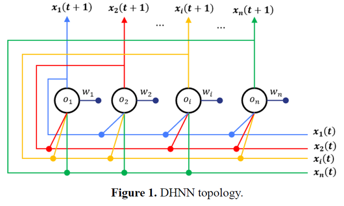
The discrete Hopfield neural network 3-satisfiability (DHNN-3SAT) model represents an innovative application of deep learning techniques to the Boolean SAT problem. Existing research indicated that the DHNN-3SAT model demonstrated significant advantages in handling 3SAT problem instances of varying scales and complexities. Compared to traditional heuristic algorithms, this model converged to local minima more rapidly and exhibited enhanced exploration capabilities within the global search space. However, the model faced several challenges and limitations. As constraints in SAT problems dynamically increased, decreased, or changed, and as problem scales expanded, the model's computational complexity and storage requirements may increase dramatically, leading to reduced performance in handling large-scale SAT problems. To address these challenges, this paper first introduced a method for designing network synaptic weights based on fundamental logical clauses. This method effectively utilized the synaptic weight information from the original SAT problem within the DHNN network, thereby significantly reducing redundant computations. Concrete examples illustrated the design process of network synaptic weights when constraints were added, removed, or updated, offering new approaches for managing the evolving constraints in SAT problems. Subsequently, the paper presented a DHNN-3SAT model optimized by genetic algorithms combined with K-modes clustering. This model employed genetic algorithm-optimized K-modes clustering to effectively cluster the initial space, significantly reducing the search space. This approach minimized the likelihood of redundant searches and reduced the risk of getting trapped in local minima, thus improving search efficiency. Experimental tests on benchmark datasets showed that the proposed model outperformed traditional DHNN-3SAT models, DHNN-3SAT models combined with genetic algorithms, and DHNN-3SAT models combined with imperialist competitive algorithms across four evaluation metrics. This study not only broadened the application of DHNN in solving 3SAT problems but also provided valuable insights and guidance for future research.
Citation: Xiaojun Xie, Saratha Sathasivam, Hong Ma. Modeling of 3 SAT discrete Hopfield neural network optimization using genetic algorithm optimized K-modes clustering[J]. AIMS Mathematics, 2024, 9(10): 28100-28129. doi: 10.3934/math.20241363
The discrete Hopfield neural network 3-satisfiability (DHNN-3SAT) model represents an innovative application of deep learning techniques to the Boolean SAT problem. Existing research indicated that the DHNN-3SAT model demonstrated significant advantages in handling 3SAT problem instances of varying scales and complexities. Compared to traditional heuristic algorithms, this model converged to local minima more rapidly and exhibited enhanced exploration capabilities within the global search space. However, the model faced several challenges and limitations. As constraints in SAT problems dynamically increased, decreased, or changed, and as problem scales expanded, the model's computational complexity and storage requirements may increase dramatically, leading to reduced performance in handling large-scale SAT problems. To address these challenges, this paper first introduced a method for designing network synaptic weights based on fundamental logical clauses. This method effectively utilized the synaptic weight information from the original SAT problem within the DHNN network, thereby significantly reducing redundant computations. Concrete examples illustrated the design process of network synaptic weights when constraints were added, removed, or updated, offering new approaches for managing the evolving constraints in SAT problems. Subsequently, the paper presented a DHNN-3SAT model optimized by genetic algorithms combined with K-modes clustering. This model employed genetic algorithm-optimized K-modes clustering to effectively cluster the initial space, significantly reducing the search space. This approach minimized the likelihood of redundant searches and reduced the risk of getting trapped in local minima, thus improving search efficiency. Experimental tests on benchmark datasets showed that the proposed model outperformed traditional DHNN-3SAT models, DHNN-3SAT models combined with genetic algorithms, and DHNN-3SAT models combined with imperialist competitive algorithms across four evaluation metrics. This study not only broadened the application of DHNN in solving 3SAT problems but also provided valuable insights and guidance for future research.

| [1] |
M. Järvisalo, B. D. Le, O. Roussel, L. Simon, The international SAT solver competitions, Ai Mag., 33 (2012), 89–92. https://doi.org/10.1609/aimag.v33i1.2395 doi: 10.1609/aimag.v33i1.2395

|
| [2] | S. A Cook, The complexity of theorem-proving procedures, Logic automata computat. Complex., 2023, 143152. |
| [3] |
J. Rintanen, Planning as satisfiability: Heuristics, Artif. Intell., 193 (2012), 45–86. https://doi.org/10.1016/j.artint.2012.08.001 doi: 10.1016/j.artint.2012.08.001
|
| [4] |
V. Popov, An approach to the design of DNA smart programmable membranes, Adv. Mater. Res., 934 (2014), 173–176. https://doi.org/10.4028/www.scientific.net/AMR.934.173 doi: 10.4028/www.scientific.net/AMR.934.173
|
| [5] |
X. Zhang, J. Bussche, F. Picalausa, On the satisfiability problem for SPARQL patterns, J. Artif. Intell. Res., 56 (2016), 403–428. https://doi.org/10.1613/jair.5028 doi: 10.1613/jair.5028
|
| [6] |
A. Armando, L. Compagna, SAT-based model-checking for security protocols analysis, Int. J. Inf. Secur., 7 (2008), 3–32. https://doi.org/10.1007/s10207-007-0041-y doi: 10.1007/s10207-007-0041-y
|
| [7] |
C. Luo, S. Cai, W. Wu, K. Su, Double configuration checking in stochastic local search for satisfiability, Proc. AAAI Conf. Artif. Intell., 28 (2014), 2703–2709. https://doi.org/10.1609/aaai.v28i1.9110 doi: 10.1609/aaai.v28i1.9110
|
| [8] |
X. Wang, A novel approach of solving the CNF-SAT problem, arXiv. Prepr. arXiv., 1307 (2013), 6291. https://doi.org/10.48550/arXiv.1307.6291 doi: 10.48550/arXiv.1307.6291
|
| [9] |
D. Karaboga, B. Gorkemli, C. Ozturk, N. Karaboga, A comprehensive survey: Artificial bee colony (ABC) algorithm and applications, Artif. Intell. Rev., 42 (2014), 21–57. https://doi.org/10.1007/s10462-012-9328-0 doi: 10.1007/s10462-012-9328-0
|
| [10] |
E. A. Hirsch, A. Kojevnikov, UnitWalk: A new SAT solver that uses local search guided by unit clause elimination, Ann. Math. Artif. Intell., 43 (2005), 91–111. https://doi.org/10.1007/s10472-005-0421-9 doi: 10.1007/s10472-005-0421-9
|
| [11] |
J. J. Hopfield, Neural networks and physical systems with emergent collective computational abilities, Proc. Natl. Acad. Sci., 79 (1982), 2554–2558. https://doi.org/10.1073/pnas.79.8.2554 doi: 10.1073/pnas.79.8.2554
|
| [12] | M. A. Mansor, S. Sathasivam, Optimal performance evaluation metrics for satisfiability logic representation in discrete Hopfield neural network, Int. J. Math. Comput. Sci., 16 (2021), 963–976. |
| [13] |
C. C. Feng, S. Sathasivam, A novel processor for dynamic evolution of constrained SAT problems: The dynamic evolution variant of the discrete Hopfield neural network satisfiability model, J. King Saud Univ., Comput. Inf. Sci., 36 (2024), 101927. https://doi.org/10.1016/j.jksuci.2024.101927 doi: 10.1016/j.jksuci.2024.101927
|
| [14] |
S. A. Karim, M. S. M Kasihmuddin, S. Sathasivam, M. A. Mansor, S. Z. M. Jamaludin, M. R. Amin, A novel multi-objective hybrid election algorithm for higher-order random satisfiability in discrete hopfield neural network, Mathematics, 10 (2022), 1963. https://doi.org/10.3390/math10121963 doi: 10.3390/math10121963
|
| [15] |
M. A. Mansor, S. Sathasivam, Accelerating activation function for 3-satisfiability logic programming, Int.J. Intell. Syst. Appl., 8 (2016), 44. https://doi.org/10.5815/ijisa.2016.10.05. doi: 10.5815/ijisa.2016.10.05
|
| [16] | S. Sathasivam, Upgrading logic programming in Hopfield network, Sains Malays., 39 (2010), 115–118. |
| [17] | M. A. Mansor, M. S. M Kasihmuddin, S. Sathasivam, Artificial immune system paradigm in the Hopfield network for 3-Satisfiability problem, Pertanika J. Sci. Technol., 25 (2017), 1173–1188. |
| [18] |
B. Bünz, M. Lamm. Graph neural networks and boolean satisfiability, arXiv. Prepr. arXiv., 1702 (2017), 03592. https://doi.org/10.48550/arXiv.1702.03592 doi: 10.48550/arXiv.1702.03592
|
| [19] |
H. Xu, S. Koenig, T. K. S. Kumar, Towards effective deep learning for constraint satisfaction problems, Int. Conf. Princ. Pract. Constraint Program., 2018,588–597. https://doi.org/10.1007/978-3-319-98334-9_38 doi: 10.1007/978-3-319-98334-9_38
|
| [20] |
H. E. Dixon, M. L. Ginsberg, Combining satisfiability techniques from AI and OR, Knowl. Eng. Rev., 15 (2000), 31–45. https://doi.org/10.1017/S0269888900001041 doi: 10.1017/S0269888900001041
|
| [21] |
W. A. Abdullah, Logic programming on a neural network, Int. J. Intell. Syst., 7 (1992), 513–519. https://doi.org/10.1002/int.4550070604 doi: 10.1002/int.4550070604
|
| [22] |
S. Sathasivam, W. A. Abdullah, Logic mining in neural network: Reverse analysis method, Computing, 91 (2011), 119–133. https://doi.org/10.1007/s00607-010-0117-9 doi: 10.1007/s00607-010-0117-9
|
| [23] |
S. Sathasivam, N. P. Fen, M. Velavan, Reverse analysis in higher order Hopfield network for higher order horn clauses, Appl. Math. Sci., 8 (2014), 601–612. http://dx.doi.org/10.12988/ams.2014.310565 doi: 10.12988/ams.2014.310565
|
| [24] |
M. S. M. Kasihmuddin, M. A. Mansor, S. Sathasivam, Discrete Hopfield neural network in restricted maximum k-satisfiability logic programming, Sains Malays., 47 (2018), 1327–1335. http:/ldx.doi.org110.17576/jsm-2018-4706-30 doi: 10.17576/jsm-2018-4706-30
|
| [25] | M. A. Mansor, M. S. M. Kasihmuddin, S. Sathasivam, Robust artificial immune system in the hopfield network for maximum k-satisfiability. Int. J. Inter. Mult. Artif. Intell., 4 (2017), 63–71. |
| [26] | M. S. M. Kasihmuddin, M. A. Mansor, S. Sathasivam, Hybrid genetic algorithm in the hopfield network for logic satisfiability problem. Pertanika J. Sci. Technol., 25 (2017), 139–152. |
| [27] |
F. L. Azizan, S. Sathasivam M. K. M. Ali, N. Roslan, C. Feng, Hybridised network of fuzzy logic and a genetic algorithm in solving 3-Satisfiability Hopfield neural networks, Axioms, 12 (2023), 250. https://doi.org/10.3390/axioms12030250 doi: 10.3390/axioms12030250
|
| [28] |
M. A. Mansor, M. S. M. Kasihmuddin, S. Sathasivam, Grey wolf optimization algorithm with discrete hopfield neural network for 3 Satisfiability analysis, J. Phys. Conf. Ser., 1821 (2021), 012038. https://doi.org/10.1088/1742-6596/1821/1/012038 doi: 10.1088/1742-6596/1821/1/012038
|
| [29] | M. A. Mansor, M. S. M. Kasihmuddin, S. Sathasivam, Modified lion optimization algorithm with discrete Hopfield neural network for higher order Boolean satisfiability programming, Malays. J. Math. Sci., 14 (2020), 47–61. |
| [30] |
N. Cao, X. J. Yin, S. T. Bai, Breather wave, lump type and interaction solutions for a high dimensional evolution model, Chaos, Solitons Fract., 172 (2023), 113505. https://doi.org/10.1016/j.chaos.2023.113505 doi: 10.1016/j.chaos.2023.113505
|
| [31] |
C. C. Feng, S. Sathasivam, N. Roslan, M. Velavan, 2-SAT discrete Hopfield neural networks optimization via Crow search and fuzzy dynamical clustering approach, AIMS Math., 9 (2024), 9232–9266. https://doi.org/10.1016/10.3934/math.2024450 doi: 10.1016/10.3934/math.2024450
|
| [32] |
S. Bai, X. Yin, N. Cao, L. Xu, A high dimensional evolution model and its rogue wave solution, breather solution and mixed solutions Nonlinear Dyn., 111 (2023), 12479–12494. https://doi.org/10.1007/s11071-023-08467-x doi: 10.1007/s11071-023-08467-x
|
| [33] |
G. He, P. Tang, X. Pang, Neural network approaches to implementation of optimum multiuser detectors in code-division multiple-access channels, Int. J. Electron., 80 (1996), 425-431. https://doi.org/10.1080/002072196137264 doi: 10.1080/002072196137264
|
| [34] |
H. Yang, Z. Li, Z. Liu, A method of routing optimization using CHNN in MANET, J. Ambient Intell. Hum. Comput., 10 (2019), 1759–1768. https://doi.org/10.1007/s12652-017-0614-1 doi: 10.1007/s12652-017-0614-1
|
| [35] |
B. Bao, H. Tang, Y. Su, H. Bao, M. Chen, Q. Xu, Two-Dimensional discrete Bi-Neuron Hopfield neural network with polyhedral Hyperchaos, IEEE Trans. Circuits Syst., (2024), 1–12. https://doi.org/10.1109/TCSI.2024.3382259 doi: 10.1109/TCSI.2024.3382259
|
| [36] |
W. Ma, X. Li, T. Yu, Z. Wang, A 4D discrete Hopfield neural network-based image encryption scheme with multiple diffusion modes, Optik, 291 (2023), 171387. https://doi.org/10.1016/j.ijleo.2023.171387 doi: 10.1016/j.ijleo.2023.171387
|
| [37] |
Q. Deng, C. Wang, H. Lin, Memristive Hopfield neural network dynamics with heterogeneous activation functions and its application, Chaos Solitons Fract., 178 (2024), 114387. https://doi.org/10.1016/j.chaos.2023.114387 doi: 10.1016/j.chaos.2023.114387
|
| [38] |
Z. S. Shazli, M. B. Tahoori, Using boolean satisfiability for computing soft error rates in early design stages, Microelectr. Reliab., 50 (2010), 149–159. https://doi.org/10.1016/j.microrel.2009.08.006 doi: 10.1016/j.microrel.2009.08.006
|
| [39] |
N. Sharma, N. Gaud, K-modes clustering algorithm for categorical data, Int. J. Comput. Appl., 127 (2015), 1–6. https://doi.org/10.1016/10.5120/ijca2015906708 doi: 10.1016/10.5120/ijca2015906708
|
| [40] |
F. Cao J. Liang, D. Li, L. Bai, C. Dang, A dissimilarity measure for the K-Modes clustering algorithm, Knowl. Based Syst., 26 (2012), 120–127. https://doi.org/10.1016/j.knosys.2011.07.011 doi: 10.1016/j.knosys.2011.07.011
|
| [41] |
M. K. Ng, M. J. Li, J. Z. Huang, Z. He, On the impact of dissimilarity measure in k-modes clustering algorithm, IEEE Trans. Pattern Anal. Mach. intell., 29 (2007), 503–507. https://doi.org/10.1109/TPAMI.2007.53 doi: 10.1109/TPAMI.2007.53
|
| [42] |
S. S. Khan, A. Ahmad, Cluster center initialization algorithm for K-modes clustering, Pattern Recognit. Lett., 25 (2004), 1293–1302. https://doi.org/10.1016/j.patrec.2004.04.007 doi: 10.1016/j.patrec.2004.04.007
|
| [43] |
R. J. Kuo, Y. R. Zheng, T. P. Q. Nguyen, Metaheuristic-based possibilistic fuzzy k-modes algorithms for categorical data clustering, Inf. Sci., 557 (2021), 1–15. https://doi.org/10.1016/j.ins.2020.12.051 doi: 10.1016/j.ins.2020.12.051
|
| [44] |
G. Gan, J. Wu, Z. Yang, A genetic fuzzy k-Modes algorithm for clustering categorical data, Expert Syst. Appl., 36 (2009), 1615–1620. https://doi.org/10.1007/11527503_23 doi: 10.1007/11527503_23
|
| [45] | F. S. Gharehchopogh, S. Haggi, An Optimization K-modes clustering algorithm with elephant herding optimization algorithm for crime clustering, J. Adv. Comput. Eng. Technol., 6 (2020), 79–90. |
| [46] |
J. Gu, Local search for satisfiability (SAT) problem, IEEE Trans. Syst., 23 (1993), 1108–1129. https://doi.org/10.1109/21.247892 doi: 10.1109/21.247892
|
| [47] |
N. E. Zamri, M. A, Mansor, M. S. M. Kasihmuddin, A. Always, S. A. Alzaeemi, Amazon employees resources access data extraction via clonal selection algorithm and logic mining approach, Entropy, 22 (2020), 596. https://doi.org/10.3390/e22060596 doi: 10.3390/e22060596
|


Figures(12) / Tables(12)

Xiaojun Xie, Saratha Sathasivam, Hong Ma. Modeling of 3 SAT discrete Hopfield neural network optimization using genetic algorithm optimized K-modes clustering[J]. AIMS Mathematics, 2024, 9(10): 28100-28129. doi: 10.3934/math.20241363


 DownLoad: