Revisiting the m-weak core inverse

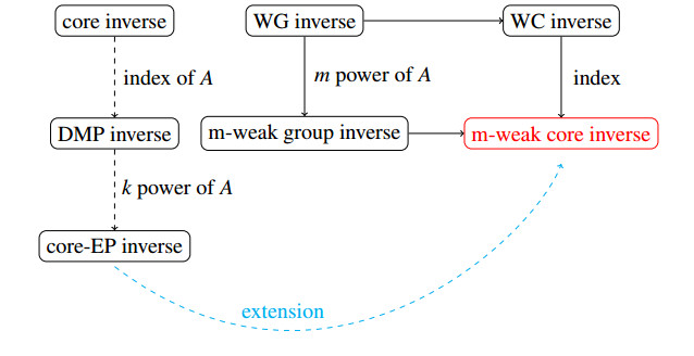
1.   Introduction

Essentially, Cohen-Grossberg neural networks (CGNNs) are a sort of artificial feedback neural networks, which means they exhibit common characteristics with other artificial neural networks in terms of information transfer and feedback mechanisms. CGNNs encompass highly adaptable neural network models (see, e.g., ^[1,2,3]), incorporating various types shaped like Hopfield neural networks and cellular neural networks, so the dynamic properties of multitudinous neural networks can be considered simultaneously when studying CGNNs. In addition, CGNNs offer extensive application prospects across various fields, including pattern recognition, classification, associative memory (see, e.g., ^[4,5,6]), etc. Stability is a prerequisite for the effectiveness of CGNNs in these applications. Thus, in order to get a larger capacity, CGNNs are designed with multiple stable equilibrium points. This has attracted many researchers to explore the multistability of CGNNs.

Actually, multistability analysis problems are typically more challenging than single-stability analysis, in which the phase space needs to be effectively partitioned into subsets containing equilibrium points according to different types of activation functions. By dividing the state space, the dynamics of multiple equilibrium points in each subset can be studied. Naturally, there are valuable works addressing this issue (see, e.g., ^{[7,8,9,10,11]}). In ^[9], Liu et al. investigated multistability in fractional-order recurrent neural networks by exploiting an activation function and nonsingular M-matrix, and they concluded that there exist ${ \prod_{i = 1}^{n}} (2K_i+1)$ equilibria, among which, ${ \prod_{i = 1}^{n}}(K_i+1)$ equilibria are local Mittag-Leffler stable. In ^[11], the authors explored multistability of CGNNs with non-monotonic activation functions and time-varying delays, and they found that one can obtain $(2K+1)^n$ equilibria for $n$-neuron CGNNs, with $(K+1)^n$ of them being exponentially stable. In addition, Wan and Liu ^[12] studied the multiple $\mathcal{O}(t^{-q})$ stability of fractional-order CGNNs with Gaussian activation functions.

To the best of our knowledge, it is agreed that the number of equilibrium points in multistability analysis of neural networks is intimately connected with the types of activation function. Some activation functions utilized widely in the existing literature are saturation function, Gaussian function, sigmoid function, Mexican-hat function ^[13], etc. Among these functions, a Gaussian function endows neural networks with greater modeling power and adaptability due to its properties of being nonmonotonic, bounded, symmetric, strongly nonlinear, and nonnegative. Additionally, research has conclusively shown that employing Gaussian activation functions in neural networks can accelerate learning and improve prediction (see, e.g., ^[14,15]). As such, it is indispensable to analyze the dynamical behavior of neural networks introducing Gaussian functions. In the literature related to Gaussian functions, Liu et al. ^[16] addressed the stable issue of recurrent neural networks with Gaussian activation functions by analyzing geometric properties of the Gaussian function. Their results concluded that there exist exactly $3^k$ equilibrium points, and $2^k$ equilibria are locally exponentially stable, while $3^k-2^k$ equilibria are unstable. In ^[17], the dynamical behaviors of multiple equilibria for fractional-order competitive neural networks with Gaussian activation functions were explored.

Due to the limited switching speeds and constrained signal propagation rates of neural amplifiers, it is imperative not to neglect time delays in neural networks (see, e.g., ^[18,19,20]). In fact, for some neurons, discrete-time delays offer a well-approximated and simplified circuit model for representing delay feedback systems. It is worth noting that neural networks typically exhibit spatial expansion since they consist of numerous parallel pathways with varying axon sizes and lengths. In such cases, the transmission of signals is not transient anymore and cannot be adequately characterized only by discrete-time delays. That is, it is reasonable to include distributed time delays in neural networks, which can reveal more realistically characteristics of neurons in the human brain (see, e.g., ^[21,22,23]). Therefore, we should be dedicated to analyzing CGNNs with mixed time delays, which is also highly necessary.

Nowadays, there are several frequently mentioned types of stability, such as asymptotic stability (see, e.g., ^[24,25]), exponential stability (see, e.g., ^[26,27]), logarithmic stability and polynomial stability ^[28]. In general, differences in stability indicate different convergence paradigms, allowing systems to satisfy the corresponding evolutionary requirements. Recently, a novel category of stability known as multimode function stability has been explored. Implementing this form of stability enables the simultaneous realization of the aforementioned types of stability. It is also revealed that multimode function stability can be employed in image processing and pattern recognition to construct neural network architectures with multiple feature extraction modes ^[29]. In ^[30], the authors presented multimode function multistability along with its specific formula. The state space was partitioned into ${ \prod_{i}^{n}} (2H_i+1)$ regions based on the positions of the zeros of boundary functions. Furthermore, through the application of the Lyapunov stability theorem and fixed point theorem, some associated criteria for multimode function multistability were obtained.

As indicated by the preceding analysis, many previous papers either analyzed only the multistability of CGNNs with/without time-varying delays and Gaussian activation functions, or solely examined the multimode function multistability of neural networks with mixed delays. There are few works on studying the multimode function multistability of CGNNs with Gaussian activation functions and mixed time delays. Consequently, we are prepared to address the multimode function multistability of CGNNs with Gaussian activation functions and mixed time delays. To be specific, the advantage of this paper can be summarized in these aspects. First, this paper will focus on specific activation functions, namely, Gaussian functions. Through the utilization of the geometrical properties of Gaussian functions, the state space can be partitioned into $3^\mu$ subspaces, where $0\le \mu\le n.$ In contrast to the class of strictly nonlinear and monotonic activation functions considered in ^[30], the number of equilibrium points in this paper is explicitly explored. Second, multimode function multistability is discussed. Quite different from most of the existing literature concerning the multistability of CGNNs with Gaussian functions, the multimode function multistability results derived herein cover multiple asymptotic stability, multiple exponential stability, multiple polynomial stability and multiple logarithmic stability, so the results presented in this paper are more universal. Finally, relying on the geometric properties of Gaussian functions and a fixed point theorem, we deduce some sufficient conditions that guarantee the coexistence of precisely $3^\mu$ equilibria for an $n$-dimensional neural network, among which $2^\mu$ equilibrium points are multimode function stable and $3^\mu-2^\mu$ equilibrium points are unstable. The results obtained here serve as a supplement to the existing relevant multimode function multistability criteria.

Notations. In this article, for a given vector $x = (x_1, x_2, ..., x_n)^T\in R^n$, define $\left \| x \right \| = \text{max}_{1\le i\le n}(|x_i|)$, and $\tilde{\tau} = \text{max}_{1\le j\le n } \biggl(\tilde{\tau}_j, \text{sup}_{t\ge0}\tau_j(t)\biggl)$. Define $\mathcal{C} ([-\tilde{\tau }, 0], \mathcal{D})$ as the Banach space of continuous functions $\phi$: $[-\tilde{\tau}, 0] \longrightarrow \mathcal{D}\subset \mathcal{R}^n$. Let $\left \| \phi \right \|_{\tilde{\tau} } = \text{max}_{1\le i\le n}(\text{sup}_{-\tilde{\tau}\le r \le 0}|\phi _i(r)|)$.

2.   Preliminaries

We introduce CGNNs with Gaussian activation functions and mixed time delays as follows:

where $x(t) = (x_1(t), x_2(t), ..., x_n(t))^T\in R^n$ is state vector. $\eta _i$ stands for the strength of self-inhibition. $m_i(\cdot)$ is amplification. $\beta _{ij}$, $\gamma _{ij}$ and $\varphi _{ij}$ are connection weights. $\tau_j(\cdot)\ge 0$ represents time-varying delay, $\tilde{\tau}_j$ in distributed delay term satisfies $\tilde{\tau}_j > 0$. $I_i$ denotes external input. $f_i(\cdot)$ is a Gaussian function with the expression:

where (2.2) satisfies $f_i(r)\in (0, 1]$, for $r\in R, c_i > 0$ represents the center and $\rho_i$ denotes the width.

The initial value of (2.1) can be written as

Prior to the study, we need to recall some definitions and consider some assumptions which will be applied in subsequent content.

Assumption 2.1. There are positive constants $\grave{m}_i$ and $\acute{M _i}$, such that

Definition 2.1. A constant vector $x^* = (x_1^*, ..., x_n^*)^T$ is regarded as an equilibrium point of (2.1), if $x^*$ satisfies

Definition 2.2. Suppose that $x_i(t)$ is the solution of neural network (2.1) with initial condition (2.3). A given set $\varTheta$ can be referred to as a positive invariant set given that, if initial condition $\phi_i(t_0)\in \varTheta$, then $x_i(t)\in \varTheta$ for all $t\ge t_0.$

Definition 2.3. Assume $x^*\in \mathcal{D}$ is an equilibrium point of (2.1), and $\mathcal{D}\subset \mathcal{R}^n$ is a positively invariant set. Furthermore, suppose that $\hbar(t)$ is a monotonically continuous and nondecreasing function for which $\hbar(t) > 0,$ for $t\ge 0, \hbar(r) = \hbar(0), r\in [-\tilde{\tau}, 0]$, and $\lim_{t\to \infty} \hbar (t) = +\infty$. If

holds for any initial value $\phi (r)\in \mathcal{D}, r\in [-\tilde{\tau}, 0]$, where $\iota > 0$ is a positive constant, then (2.1) is locally multimode function stable.

Calculating the first and second-order derivatives of activation function $f_i(r)$:

we can find $f_i' (r)$ has one root $r_i = c_i$ via solving the equation $f_i' (r) = 0$. Analogously, by addressing the equation $f_i''(r) = 0$, we can gain two roots of $f_i''(r)$:

For $r\in (-\infty, C_i^-)\cup (C_i^+, +\infty),$ $f_i'' (r) > 0,$ with regard to $r\in (C_i^-, C_i^+),$ $f_i'' (r) < 0,$ we can conclude that $C_i^-$ and $C_i^+$ are the maximum and minimum points of $f_i' (r)$, separately. The maximum and minimum values of $f_i' (r)$ are $f_i' (C_i^-) = \sqrt{2}\text{exp}(-1/2)/\rho_i, f_i' (C_i^+) = -\sqrt{2}\text{exp}(-1/2)/\rho_i$, respectively. For the convenience of discussion, we define $\delta _i = \sqrt{2}\text{exp}(-1/2)/\rho_i, i = 1, 2, ..., n.$

Since $f_i(r)\in (0, 1]$ for all $i = 0, 1, ..., n,$ let

Define the boundary functions:

and simultaneously, we define

where $\bar{s}_i\in(\check{s}_i, \hat{s}_i)$ is a constant. Then $W^-_i(x_i(t)),$ $\bar {W}_i(x_i(t)),$ and $W^+_i(x_i(t))$ are vertical shifts toward each other.

Let $\mathcal{N} = \left \{ 1, 2, ..., n \right \}$. According to the specific values of the parameters $\eta_i$ and $\beta_{ii}$, define

Lemma 2.1 (^[16]). If $i\in \mathcal{L}_1$ or $\mathcal{L}_3$, then there are $p_i, q_i$ such that $\bar{W}_i'(p_i) = {\bar{W}_i}'(q_i) = 0$, where $p_i < R_i^- < q_i < c_i,$ if $i\in \mathcal{L}_2$ or $\mathcal{L}_4$, then ${\bar{W}_i}'(r) < 0$ for $r\in\mathcal{R}$.

For the sake of discussion, the subsequent subsets of $\mathcal{L}_1$ and $\mathcal{L}_3$ are considered:

Lemma 2.2 (^[16]). If $i\in \mathcal{L}_1^1\cup \mathcal{L}_3^1$, then there exist three zeros $\check{u}_i, \check{v}_i, \check{\lambda}_i$ for $W^-_i(r)$ and three zeros $\hat{u}_i, \hat{v}_i, \hat{\lambda}_i$ for $W^+_i(r)$, satisfying $\check{u}_i < \hat{u}_i < p_i < \hat{v}_i < \check{v}_i < q_i < \check{\lambda}_i < \hat{\lambda}_i$.

If $i\in \mathcal{L}_1^2\cup \mathcal{L}_3^2$, then there exists one zero $\check{o}_i$ for $W^-_i(r)$, and one zero $\hat{o}_i$ for $W^+_i(r)$, satisfying $\check{o}_i < \hat{o}_i < p_i.$

If $i\in \mathcal{L}_1^3\cup \mathcal{L}_3^3$, then there exists one zero $\check{o}_i$ for $W^-_i(r)$, and one zero $\hat{o}_i$ for $W^+_i(r)$, satisfying $q_i < \check{o}_i < \hat{o}_i.$

If $i\in \mathcal{L}_2\cup \mathcal{L}_4$, then there exists one zero $\check{o}_i$ for $W^-_i(r)$, and one zero $\hat{o}_i$ for $W^+_i(r)$, satisfying $\check{o}_i < \hat{o}_i.$

3.   Main results

3.1.   Equilibrium points

In what follows, the number of equilibrium points of (2.1) is explored. Let card $\mathcal{Q}$ represent the cardinality of a given set $\mathcal{Q}$. Define $\mu$ = card$(\mathcal{L}_1^1\cup \mathcal{L}_3^1)$, $k$ = card $(\mathcal{L}_1^2\cup \mathcal{L}_1^3\cup \mathcal{L}_2\cup \mathcal{L}_3^2\cup \mathcal{L}_3^3\cup \mathcal{L}_4),$ and let

The following assumption is required so as to ascertain the number of equilibrium points of (2.1).

Assumption 3.1. $k+\mu = n.$

Consequently, it can be seen that there exist $3^\mu$ elements in $\Theta$.

Theorem 3.1. Suppose Assumption 3.1 holds. Further assume that

where $i\in \mathcal{N}$, and $\mathcal{F}_i$ is given in Table 1. Then, neural network (2.1) has accurately $3^\mu$ equilibria in $\mathcal{R}^n$.

Proof. We first demonstrate the existence of equilibrium points of (2.1) for any $\Theta ^{(1)} = \prod_{i = 1}^{n} l_i = \prod_{i = 1}^{n}[d_i, g_i]\in \Theta$.

With regard to any given $x = (x_1, x_2, ..., x_n)^T$ and index $i\in \mathcal{N}$, define the following function:

Comparing $W_i(r)$ with $W^+_i(r), W^-_i(r)$, we can get that $W^-_i(r)\le W_i(r)\le W^+_i(r)$ for $r\in[d_i, g _i]$. Then, two cases will be considered.

Case 1: when $l_i = [\hat{v}_i, \check{v}_i],$ we can obtain

Case 2: when $l_i\ne [\hat{v}_i, \check{v}_i],$ we get

Taken together, $W_i(d _i)W_i(g_i)\le 0$, whereupon there exists a $\bar{x}_i\in [d_i, g _i]$ satisfying $W_i(\bar{x}_i) = 0$ for $i = 1, 2, ..., n.$ Define a continuous mapping $\Xi$ : $\Theta^{(1)} \rightarrow \Theta^{(1)}$, $\Xi(x_1, x_2, ..., x_n) = (\bar{x}_1, \bar{x}_2, ..., \bar{x}_n)^T$. By virtue of a fixed point theorem, we can assert the existence of a fixed point $x^* = (x_1^*, x_2^*, ..., x_n^*)^T$ of $\Xi$, which also serves as an equilibrium point for (2.1).

Following that, we are prepared to certify the uniqueness of equilibrium points in $\Theta^{(1)}$. For any $x, y\in \Theta^{(1)}$, hypothesize that $\Xi(x) = x^*, \Xi(y) = y^*$ and $x^*, y^*$ are both roots of $W_i(r)$.

Hence,

Subtracting (3.3) from (3.2), it follows that

where $\text{min}(x_i^*, y_i^*)\le \xi_i^*\le \text{max}(x_i^*, y_i^*)$. In the following, eight situations are discussed.

Case 1: $i\in \mathcal{L}_1^1$.

If $\xi_i^*\in [\check{u}_i, \hat{u}_i]$, we have $f_i'(\xi_i^*)\le \frac{\eta _i}{\beta_{ii}}$ and $0 < f_i'(\check{u}_i)\le f_i'(\xi_i^*)\le f_i'(\hat{u}_i);$ hence

If $\xi_i^*\in [\hat{v}_i, \check{v}_i]$, we can get $f_i'(\xi_i^*)\ge \frac{\eta _i}{\beta_{ii}}$, and $0 < \text{min}\left\{f_i'(\check{v}_i), f_i'(\hat{v}_i)\right\}\le f_i'(\xi_i^*)\le \delta_i$, then

If $\xi_i^*\in [\check{\lambda}_i, \hat{\lambda}_i]$, we can obtain $f_i'(\xi_i^*)\le \frac{\eta _i}{\beta_{ii}}$, and $-\delta _i\le f_i'(\xi_i^*)\le \text{max}\left\{f_i'(\check{\lambda}_i), f_i'(\hat{\lambda}_i)\right\},$ then

Case 2: $i\in \mathcal{L}_1^2$. In this case, $\xi_i^*\in [\check{o}_i, \hat{o}_i]$, we can know $f_i'(\xi_i^*)\le \frac{\eta _i}{\beta_{ii}}$, and $0 < f_i'(\check{o}_i)\le f_i'(\xi_i^*)\le f_i'(\hat{o}_i).$ Hence,

Case 3: $i\in \mathcal{L}_1^3$. In this case, $f_i'(\xi_i^*)\le \frac{\eta _i}{\beta_{ii}}$ and $f_i'(\xi_i^*)\le \text{max}\left\{f_i'(\check{o}_i), f_i'(\hat{o}_i)\right\}.$ Hence,

Case 4: $i\in \mathcal{L}_2$. In this case, $\xi_i^*\in [\check{o}_i, \hat{o}_i], f_i'(\xi_i^*)\le \delta_i < \frac{\eta _i}{\beta_{ii}},$ so we can get

Case 5: $i\in \mathcal{L}_3^1$.

If $\xi_i^*\in [\check{u}_i, \hat{u}_i]$, we have $\beta_{ii} < 0,$ $f_i'(\xi_i^*)\ge \frac{\eta _i}{\beta_{ii}}$, and $\text{min}\left\{f_i'(\check{u}_i), f_i'(\hat{u}_i)\right\}\le f_i'(\xi_i^*)\le \delta_i.$ Hence,

If $\xi_i^*\in [\hat{v}_i, \check{v}_i]$, we can get $\beta_{ii} < 0, f_i'(\xi_i^*)\le \frac{\eta _i}{\beta_{ii}}$, and $-\delta_i\le f_i'(\xi_i^*)\le \text{max}\left\{f_i'(\check{v}_i), f_i'(\hat{v}_i)\right\} < 0$. Then,

If $\xi_i^*\in [\check{\lambda}_i, \hat{\lambda}_i]$, we can obtain $\beta_{ii} < 0, f_i'(\xi_i^*)\ge \frac{\eta _i}{\beta_{ii}}$, and $f_i'(\check{\lambda}_i)\le f_i'(\xi_i^*)\le f_i'(\hat{\lambda}_i) < 0.$ Then,

Case 6: $i\in \mathcal{L}_3^2$. In this case, $\beta_{ii} < 0, \xi_i^*\in [\check{o}_i, \hat{o}_i]$. We can know $f_i'(\xi_i^*)\ge \frac{\eta _i}{\beta_{ii}}$, and $\text{min}\left\{f_i'(\check{o}_i), f_i'(\hat{o}_i)\right\}\le f_i'(\xi_i^*)\le \delta_i.$ Hence,

Case 7: $i\in \mathcal{L}_3^3$. In this case, $\beta_{ii} < 0, f_i'(\xi_i^*)\ge \frac{\eta _i}{\beta_{ii}}$ and $f_i'(\check{o}_i)\le f_i'(\xi_i^*)\le f_i'(\hat{o}_i) < 0.$ Hence,

Case 8: $i\in \mathcal{L}_4$. In this case, $\beta_{ii} < 0, \xi_i^*\in [\check{o}_i, \hat{o}_i],$ and $f_i'(\xi_i^*)\ge -\delta_i > \frac{\eta _i}{\beta_{ii}},$ so we can get

Based on the above discussion,

where $\Delta = \text{max}_{1\le i\le n}(\frac{\sum_{j = 1, j\ne i}^{n}\delta_j |\beta_{ij}|+\sum_{j = 1}^{n} \delta_j |\gamma _{ij}| +\sum_{j = 1}^{n} \delta_j |\varphi _{ij}|\tilde{\tau}_j}{\mathcal{F}_i})$, and $\mathcal{F}_i$ is described in Table 1.

Recalling (3.1), $\Delta < 1$. Consequently, $\Xi$ is a contraction mapping in $\Theta^{(1)}\in \Theta$. Hence, a unique equilibrium point exists within $\Theta^{(1)}$. From Assumption 3.1, the number of elements of $\Theta$ is $3^\mu$, so the neural network (2.1) has exactly $3^\mu$ unique equilibrium points. □

3.2.   Multimode function multistability

From the discussion in the preceding subsection, we have obtained that there are exactly $3^\mu$ equilibrium points. In this subsection, we will inquire into the multimode function stability of $3^\mu$ equilibria for CGNNs with Gaussian activation functions and mixed time delays. For this purpose, the invariant set needs to be specified.

Define

where $0 < \varrho < \text{min}_{1\le i\le n}(\varrho_i)$, and define

Let $\Theta_{(1)}^{\varrho} = { \prod_{i = 1}^{n}}[\check{\partial}i-\varrho, \hat{\partial}i+\varrho]$ and $\check{\Theta}_{(1)}^{\varrho} = { \prod_{i = 1}^{n}}[\check{\epsilon}_i-\varrho, \hat{\epsilon}_i+\varrho]$ be elements of $\Theta_i^{\varrho}$ and $\check{\Theta}_i^{\varrho}$, respectively.

Remark 3.1. Under the condition of Theorem 3.1, it is observed that there are exactly $2^\mu$ elements in $\Theta_i^{\varrho}$ and $3^\mu-2^\mu$ elements in $\check{\Theta}_i^{\varrho}$.

Theorem 3.2. Suppose Assumption 3.1 holds. Then, $\Theta_{(1)}^{\varrho}\in \Theta_i^{\varrho}$ is a positive invariant set for initial state of (2.1) with $\phi_i(t_0)\in \Theta_{(1)}^{\varrho}$.

Proof. For any initial value $\phi_i (s)\in \mathcal{C} ([-\tilde{\tau }, 0], \mathcal{D})$, if $\phi_i (t_0)\in [\check{\partial }_i-\varrho, \hat{\partial }_i+\varrho]$, we require that the corresponding solution $x_i(t)$ of (2.1) meets $x_i(t)\in[\check{\partial }_i-\varrho, \hat{\partial }_i+\varrho]$ for all $t\ge t_0$. Otherwise, there must exist an index $i$, $t_2 > t_1 > t_0$, and $\omega$ which is an adequately small positive number, such that

On the other hand, it is not difficult to observe that for any element $[\check{\partial }_i-\varrho, \hat{\partial }_i+\varrho]\in \Theta_i^{\varrho}$, $W^+_i(\hat{\partial }_i+\varrho) < 0$, then

This is in contradiction to $x_i'(t_1)\ge 0$. Then, $x_i(t)\le \hat{\partial }_i+\varrho$. Likewise, we can prove that $x_i(t)\ge \check{\partial }_i-\varrho$, for $t\ge t_0$ and $i = 1, 2, ..., n.$ Accordingly, each set in $\Theta_i^{\varrho}$ is a positive invariant set. □

Remark 3.2. From Remark 3.1, there exist $2^\mu$ elements in $\Theta_i^{\varrho}$, so the number of positively invariant sets is $2^\mu$ for initial state $\phi_i(t_0)\in \Theta_{(1)}^{\varrho}$ of neural network (2.1).

Below, we will investigate whether the equilibria located in the positive invariant sets are multimode function stable for neural network (2.1). For this reason, we need to introduce the following assumption and lemma.

Assumption 3.2. $\hbar(t)$ is a monotonically continuous and non-decreasing function. It satisfies $\hbar(t) > 0$ for $t\ge 0,$ and $\hbar(r) = \hbar(0), r\in [-\tilde{\tau}, 0]$. Further suppose

holds, where $P(\cdot)$ is a monotonically nondecreasing nonnegative function, and $\varepsilon > 0$ is a constant.

Hence, it is easy to obtain that $\frac{\mathrm{d} \hbar (t)}{\mathrm{d} t} /\hbar (t)\le \varepsilon$.

Lemma 3.1 ^[26]. Suppose that Assumption 3.2 holds. Then,

where $\zeta \in[-\tilde{\tau}, 0]$ is a constant.

Let $x^*\in \Theta_{(1)}^{\varrho}$ be an equilibrium point of (2.1). Define

where $x(t) = (x_1(t), x_2(t), ..., x_n(t))^T$ is the solution of neural network (2.1) and its initial condition $\phi (r)\in \Theta_{(1)}^{\varrho}, r\in [-\tilde{\tau}, 0]$.

Thereupon,

For convenience, let $F_i(t) = f_i(\upsilon _i(t)+x_i^*)-f_i(x_i^*)$. Hence, from (3.5)

Consider the following expression:

When $i\in \mathcal{L}_1^1,$ if $l_i = [\check{u}_i-\varrho, \hat{u}_i+\varrho],$

and if $l_i = [\check{\lambda}_i-\varrho, \hat{\lambda}_i+\varrho]$,

When $i\in \mathcal{L}_1^2$, $l_i = [\check{o}_i-\varrho, \hat{o}_i+\varrho]$,

When $i\in \mathcal{L}_1^3$, $l_i = [\check{o}_i-\varrho, \hat{o}_i+\varrho]$,

When $i\in \mathcal{L}_2\cup \mathcal{L}_4$, $l_i = [\check{o}_i-\varrho, \hat{o}_i+\varrho]$, $-\delta_i\le \frac{F_i(t)}{\upsilon _i(t)}\le \delta_i.$

When $i\in \mathcal{L}_3^1,$ if $l_i = [\check{u}_i-\varrho, \hat{u}_i+\varrho],$

if $l_i = [\check{\lambda}_i-\varrho, \hat{\lambda}_i+\varrho]$,

When $i\in \mathcal{L}_3^2$, $l_i = [\check{o}_i-\varrho, \hat{o}_i+\varrho]$,

When $i\in \mathcal{L}_3^3$, $l_i = [\check{o}_i-\varrho, \hat{o}_i+\varrho]$,

Taking into account these cases, we can get

where $\Psi _i$ is described in Table 2.

Theorem 3.3. Assume the conditions of Assumptions 2.1–3.2 are satisfied. Further suppose that there are $n$ positive constants $\sigma_1, \sigma_2, ..., \sigma_n$ such that

holds for $i = 1, 2, ..., n.$ Then, there are $2^\mu$ equilibria which are locally multimode function stable, and $3^\mu-2^\mu$ equilibrium points are unstable in (2.1).

Proof. Based on the analysis in the previous subsection, there exist exactly $2^\mu$ equilibria in $\Theta_i^{\varrho}$. Our objective now is simply to prove $2^\mu$ equilibria are multimode function stable in $\Theta_i^{\varrho}$, while other equilibria in $\check{\Theta}_i^{\varrho}$ are unstable.

Take

and there must be some $\kappa\in \left \{ 1, 2, ..., n \right \}$ such that $\varpi (t) = \frac{\left | \upsilon _\kappa(t) \right |}{\sigma_\kappa }.$

Under (3.6), we get

Note that

and

Combining with the above calculation and (3.7), we can obtain

By invoking (3.9),

From Lemma 3.1,

Hence,

In the following, it is demanded that

and if not, there must be certain $\mathcal{T}^* > 0$ satisfying

In other words,

which means that

From the above discussion and (3.10), we can derive

The result contradicts with (3.12). Hence, (3.11) holds, which implies

where $\iota = \frac{\hat{\sigma }\hbar (0) }{\check{\sigma } }, \ \hat{\sigma } = \text{max}_{1\le i\le n}(\sigma_i), \ \check{\sigma } = \text{min}_{1\le i\le n}(\sigma_i).$ The proof is accomplished. □

4.   Numerical examples

We offer two numerical examples of 2-dimensional CGNNs with Gaussian activation functions and mixed time delays to show the efficacy of theoretical results in this subsection.

Example 4.1. Consider the 2-dimensional CGNNs with Gaussian activation functions and mixed time delays presented below:

where Gaussian activation functions $f_1(r) = f_2(r) = \text{exp}(-r^2),$ $\tau_1(t) = 1.5+\text{cos}(t), \tau_2(t) = \frac{2t}{1+t}, \tilde{\tau}_1 = 1.1, \tilde{\tau}_2 = 1.2.$

It can be gained apparently that

Since $m_1(x_1(t)) = 4+\text{sin}(x_1(t))\in [3, 5],$ $m_2(x_2(t)) = 5+\text{sin}(x_2(t))\in [4, 6],$ Assumption 2.1 is met. Moreover $\tilde{\tau} = 2.5,$ $\check{s}_1 = -2.53,$ $\hat{s}_1 = -2.276,$ $\check{s}_2 = -3.01,$ $\hat{s}_2 = -2.829.$ Hence, the boundary functions are as follows:

where the graphs of these boundary functions are described as Figures 1 and 2.

Additionally,

which demonstrates that $1\in \mathcal{L}_1, 2\in \mathcal{L}_2$.

By means of further calculations, we can obtain that $\mu = 1$. $\check{u}_1\approx-2.5270,$ $\hat{u}_1\approx-2.2570,$ $\check{v}_1\approx-0.9550,$ $\hat{v}_1\approx -0.8480,$ $\check{\lambda}_1\approx0.3629,$ $\hat{\lambda}_1\approx0.4364,$ $p_1\approx-1.5261,$ $q_1\approx-0.1441.$ Also, ${W}^+_1(p_1) = -0.4285 < 0, {W}^-_1(q_1) = 0.8463 > 0.$ Therefore, $1\in \mathcal{L}_1^1$.

Furthermore, $\check{o}_2\approx-3.0699,$ $\hat{o}_2\approx-2.8286.$ $f_1'(\check{v}_1) = 0.6621,$ $f_1'(\hat{v}_1) = 0.4270,$ $f_1'(\hat{u}_1) = 0.1131,$ $f_1'(\check{\lambda}_1) = -1.2914,$ $f_1'(\hat{\lambda}_1) = -1.0235.$ By computation, $\mathcal{F}_1\approx0.4091,$ $\mathcal{F}_2\approx0.2564.$

Then,

are met. Hence, depending on Theorem 3.1, there are 3 equilibria for (4.1). By applying MATLAB, we find that these equilibrium points are (-0.8174, -2.4286), (-2.4930, -2.4979), and (0.3674, -2.3795), respectively.

Moreover, $\varrho_1 = \text{min}(p_1-\hat{u}_1, \check{\lambda}_1-q_1)\approx 0.5070,$ $\varrho_2 = 1,$ so let $\varrho = 0.1.$ From Theorem 3.2, there exist two positively invariant sets, which are $[-2.627, -2.156]\times [-3.1699, -2.7286],$ and $[0.3529, 0.5364]\times [-3.1699, -2.7286]$.

Next, we need to check out the stability condition (3.8) in Theorem 3.3. Select $\sigma _1 = \sigma _2 = 1,$ $\Psi_1 = \text{max}{(f_1'(\hat{u}_i+\varrho), f_1'(\check{\lambda}_1-\varrho)\approx0, f_1'(\hat{\lambda}_1+\varrho))} = 0.1589,$ $\Psi_2\approx0$ Now, we let $\hbar (t)$ be an exponential function with the expression $\hbar (t) = \text{exp}(0.06t),$ so $\varepsilon = 0.06$. By further calculating

The result shows that (3.8) holds, that is, the equilibrium points $(-2.4930, -2.4979)$ and $(0.3674, -2.3795)$ are multimode function stable, whereas the equilibrium point $(-0.8174, -2.4286)$ is unstable. The trajectory behavior of (4.1) and the equilibrium points are illustrated by Figures 3–5.

Example 4.2. Consider the 2-dimensional CGNNs with Gaussian activation functions and mixed time delays presented below:

where Gaussian activation functions $f_1(r) = f_2(r) = \text{exp}(-r^2),$ $\tau_1(t) = 1+0.5\text{sin}(t), \tau_2(t) = \frac{t}{1+t}, \tilde{\tau}_1 = 1.15, \tilde{\tau}_2 = 1.22.$

It can be gained apparently that

Since $m_1(x_1(t)) = 2+\text{sin}(x_1(t))\in [1, 3],$ $m_2(x_2(t)) = 4+\text{cos}(x_2(t))\in [3, 5],$ Assumption 2.1 is met. Moreover $\tilde{\tau} = 1.5,$ $\check{s}_1 = -4.5,$ $\hat{s}_1 = -3.7756,$ $\check{s}_2 = -5,$ $\hat{s}_2 = -4.217.$ Hence, the boundary functions are as follows:

where the graphs of these boundary functions are portrayed in Figures 6 and 7.

Additionally,

which implies that $1\in \mathcal{L}^1_1, 2\in \mathcal{L}^1_1$, and $\mu = 2$.

By means of further calculations, $\check{u}_1\approx-4.5,$ $\hat{u}_1\approx-3.7756,$ $\hat{v}_1\approx-0.8821,$ $\check{v}_1\approx -0.7135,$ $\check{\lambda}_1\approx0.4841,$ $\hat{\lambda}_1\approx0.6031,$ $p_1\approx-1.7400,$ $q_1\approx-0.1230.$ Also, $\check{u}_2\approx-5,$ $\hat{u}_2\approx-4.217,$ $\hat{v}_2\approx-0.9039,$$\check{v}_2\approx -0.7543,$ $\check{\lambda}_2\approx0.5489,$ $\hat{\lambda}_2\approx0.6566,$ $p_2\approx-1.8380,$ $q_2\approx-0.02.$

Furthermore, $f_1'(\check{v}_1)\approx0.8577,$ $f_1'(\hat{v}_1)\approx0.8103,$ $f_1'(\hat{u}_1)\approx0,$ $f_1'(\check{\lambda}_1)\approx-0.7659,$ $f_1'(\hat{\lambda}_1)\approx-0.8384$, $f_2'(\check{v}_1)\approx0.7986,$ $f_2'(\hat{v}_1)\approx0.8540,$ $f_2'(\hat{u}_1)\approx0,$ $f_2'(\check{\lambda}_1)\approx-0.8122,$ $f_2'(\hat{\lambda}_1)\approx-0.8533$. By computation, $\mathcal{F}_1 = 1,$ $\mathcal{F}_2 = 1.5.$ Then,

are met. Hence, according to Theorem 3.1, there are $3^2 = 9$ equilibrium points for (4.2). Moreover, $\varrho_1 = \text{min}(p_1-\hat{u}_1, \check{\lambda}_1-q_1)\approx 0.6071,$ $\varrho_2 = \text{min}(p_2-\hat{u}_2, \check{\lambda}_2-q_2)\approx0.5689,$ so let $\varrho = 0.1.$ From Theorem 3.2, there exist four positively invariant sets, which are $[-4.6, -3.6756]\times [-5.1, -4217],$ $[0.3841, 0.7031]\times [-5.1, -4217],$ $[-4.6, -3.6756]\times [0.4489, 0.7566],$ $[0.3841, 0.7031]\times [0.4489, 0.7566].$ By applying MATLAB, the stable equilibrium points are (-4.441, -2.639), (0.498, -2.355), (0.5126, 0.7593), and (-4.193, 0.6693), respectively.

Next, we need to check out the stability condition (3.8) of Theorem 3.3. Select $\sigma _1 = \sigma _2 = 1,$ $\Psi_1 = \text{max}{(f_1'(\hat{u}_i+\varrho), f_1'(\check{\lambda}_1-\varrho), f_1'(\hat{\lambda}_1+\varrho))},$ $\Psi_2 = 0.8578.$ Now, we let $\hbar (t)$ be a logarithmic function, where $P (t) = \text{ln}(t+8.0101),$ $\varepsilon = 0.5$, so $\hbar(t) = 0.5-\frac{1}{(t+8.0101)\text{ln}(t+8.0101)}.$ By further calculating

The result shows that (3.8) holds, that is, equilibrium points (-4.441, -2.639), (0.498, -2.355), (0.5126, 0.7593), and (-4.193, 0.6693) are multimode function stable. The trajectory behavior of (4.2) as well as the equilibrium points in this case are portrayed by Figures 8–10.

5.   Conclusions

In this paper, we probe into multimode function multistability of CGNNs with Gaussian activation functions and mixed time delays. Specifically, on account of the special geometric properties of Gaussian functions, the state space of an $n$-dimensional CGNNs can be divided into $3^\mu$ subspaces ($0\le \mu\le n$), further exploiting Brouwer's fixed point theorem and contraction mapping, we conclude that there exists an equilibrium point for each subspace, that is, there are exactly $3^\mu$ equilibria for CGNNs with Gaussian activation functions and mixed time delays. Subsequently, by analyzing the invariance sets, it is deduced that $2^\mu$ equilibrium points are multimode function stable, while $3^\mu-2^\mu$ equilibrium points are unstable. This work extends the existing results concerning the multistability of multimode functions, offering effective assistance in the dynamic analysis of CGNNs with specific activation functions and mixed time delays.

Use of AI tools declaration

The authors declare they have not used Artificial Intelligence (AI) tools in the creation of this article.

Conflict of interest

The authors declare that there are no conflicts of interest.