A novel delayed exponent coupled chaotic map with countering dynamical degradation

Bowen Zhang; Lingfeng Liu; Bowen Zhang; Lingfeng Liu

doi:10.3934/math.2024007

AIMS Mathematics

2024, Volume 9, Issue 1: 99-121. doi: 10.3934/math.2024007

Previous Article Next Article

Research article

A novel delayed exponent coupled chaotic map with countering dynamical degradation

Bowen Zhang ,
Lingfeng Liu ^,

School of Software, Nanchang University, Nanchang 330031, China

Received: 08 October 2023 Revised: 14 November 2023 Accepted: 21 November 2023 Published: 27 November 2023
MSC : 34H10, 37G15

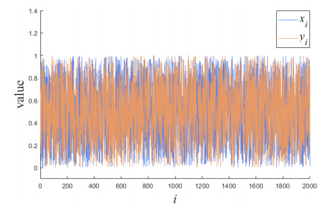
While chaotic systems have found extensive applications across diverse scientific domains due to their inherent advantages, they often degrade into cyclic patterns when simulated on hardware with limited computational precision. This results in a pronounced decline in properties related to chaotic dynamics. To address this issue, we introduce the delayed exponent coupled chaotic map (DECCM). This model is designed to enhance the chaotic dynamics of the original map, especially at lower computational precisions. Additionally, DECCM can transform any proficient 1-dimensional seed map into an N-dimensional chaotic map. Extensive simulation and performance tests attest to the robust chaotic characteristics of our approach. Furthermore, DECCM holds distinct advantages over premier algorithms, particularly in period analysis experiments. We also introduce various seed maps into DECCM to present 2D and 3D examples, ensuring their generalization through relevant performance evaluations.

Keywords:

Citation: Bowen Zhang, Lingfeng Liu. A novel delayed exponent coupled chaotic map with countering dynamical degradation[J]. AIMS Mathematics, 2024, 9(1): 99-121. doi: 10.3934/math.2024007

Related Papers:

[1]	Siting Yu, Jingjing Peng, Zengao Tang, Zhenyun Peng . Iterative methods to solve the constrained Sylvester equation. AIMS Mathematics, 2023, 8(9): 21531-21553. doi: 10.3934/math.20231097
[2]	Nunthakarn Boonruangkan, Pattrawut Chansangiam . Convergence analysis of a gradient iterative algorithm with optimal convergence factor for a generalized Sylvester-transpose matrix equation. AIMS Mathematics, 2021, 6(8): 8477-8496. doi: 10.3934/math.2021492
[3]	Jin-Song Xiong . Generalized accelerated AOR splitting iterative method for generalized saddle point problems. AIMS Mathematics, 2022, 7(5): 7625-7641. doi: 10.3934/math.2022428
[4]	Jiaxin Lan, Jingpin Huang, Yun Wang . An E-extra iteration method for solving reduced biquaternion matrix equation $AX+XB = C$ . AIMS Mathematics, 2024, 9(7): 17578-17589. doi: 10.3934/math.2024854
[5]	Kanjanaporn Tansri, Pattrawut Chansangiam . Gradient-descent iterative algorithm for solving exact and weighted least-squares solutions of rectangular linear systems. AIMS Mathematics, 2023, 8(5): 11781-11798. doi: 10.3934/math.2023596
[6]	Yinlan Chen, Min Zeng, Ranran Fan, Yongxin Yuan . The solutions of two classes of dual matrix equations. AIMS Mathematics, 2023, 8(10): 23016-23031. doi: 10.3934/math.20231171
[7]	Wenxiu Guo, Xiaoping Lu, Hua Zheng . A two-step iteration method for solving vertical nonlinear complementarity problems. AIMS Mathematics, 2024, 9(6): 14358-14375. doi: 10.3934/math.2024698
[8]	Wen-Ning Sun, Mei Qin . On maximum residual block Kaczmarz method for solving large consistent linear systems. AIMS Mathematics, 2024, 9(12): 33843-33860. doi: 10.3934/math.20241614
[9]	Kanjanaporn Tansri, Sarawanee Choomklang, Pattrawut Chansangiam . Conjugate gradient algorithm for consistent generalized Sylvester-transpose matrix equations. AIMS Mathematics, 2022, 7(4): 5386-5407. doi: 10.3934/math.2022299
[10]	Yang Cao, Quan Shi, Sen-Lai Zhu . A relaxed generalized Newton iteration method for generalized absolute value equations. AIMS Mathematics, 2021, 6(2): 1258-1275. doi: 10.3934/math.2021078

Abstract

1. Introduction

Fractional calculus deals with the equations which involve integrals and derivatives of fractional orders. The history of fractional calculus begins from the history of calculus. The role of fractional integral operators is very vital in the applications of this subject in other fields. Several well known phenomenas and their solutions are presented in fractional calculus which can not be studied in ordinary calculus. Inequalities are useful tools in mathematical modelling of real world problems, they also appear as constraints to initial/boundary value problems. Fractional integral/derivative inequalities are of great importance in the study of fractional differential models and fractional dynamical systems. In recent years study of fractional integral/derivative inequalities accelerate very fastly. Many well known classical inequalities have been generalized by using classical and newly defined integral operators in fractional calculus. For some recent work on fractional integral inequalities we refer the readers to ^{[1,2,3,4,5,6]} and references therein.

Our goal in this paper is to apply generalize Riemann-Liouville fractional integrals using a monotonically increasing function. The Hadamard inequalities are proved for these integral operators using strongly $(\alpha, m)$ -convex functions. Also error bounds of well known Hadamard inequalities are obtained by using two fractional integral identities. In connection with the results of this paper, we give generalizations and refinements of some well known results added recently in the literature of mathematical inequalities.

Next, we like to give some definitions and established results which are necessary and directly associated with the findings of this paper.

Definition 1. ^[7] A function $f: [0, +\infty)\rightarrow \mathbb{R}$ is said to be strongly $(\alpha, m)$ -convex function with modulus $c\geq0$ , where $(\alpha, m)\in [0, 1]^{2}$ , if

$\begin{equation} f(xt+m(1-t)y)\leq t^{\alpha}f(x)+m(1-t^{\alpha})f(y)-cmt^{\alpha}(1-t^{\alpha})|y-x|^{2}, \end{equation}$

(1.1)

holds $\forall\, \, x, y\in [0, +\infty)$ and $t\in[0, 1]$ .

The well-known Hadamard inequality is a very nice geometrical interpretation of convex functions defined on the real line, it is stated as follows:

Theorem 1. The following inequality holds:

$\begin{align} f\left(\frac{x+y}{2}\right)\leq\frac{1}{y-x}\int_{x}^{y}f(v)dv\leq\frac{f(x)+f(y)}{2}, \end{align}$

(1.2)

for convex function $f:I\rightarrow \mathbb{R}$ , where $I$ is an interval and $x, y \in I$ , $x < y$ .

The definition of Riemann-Liouville fractional integrals is given as follows:

Definition 2. Let $f\in L_{1}[a, b]$ . Then left-sided and right-sided Riemann-Liouville fractional integrals of a function $f$ of order $\mu$ where $\Re(\mu) > 0$ are defined by

$\begin{equation} I_{a^+}^{\mu}f(x) = \frac{1}{\Gamma({\mu})}\int_{a}^{x}(x-t)^{\mu-1}f(t)dt, \quad x > a, \end{equation}$

(1.3)

and

$\begin{equation} I_{b^-}^{\mu}f(x) = \frac{1}{\Gamma({\mu})}\int_{x}^{b}(t-x)^{\mu-1}f(t)dt, \quad x < b. \end{equation}$

(1.4)

The following theorems provide two Riemann-Liouville fractional versions of the Hadamard inequality for convex functions.

Theorem 2. ^[8] Let $f:[a, b] \rightarrow \mathbb{R}$ be a positive function with $0\leq a < b$ and $f\in L_{1}[a, b]$ . If $f$ is a convex function on $[a, b]$ , then the following fractional integral inequality holds:

$\begin{align} & f\left(\frac{a+b}{2}\right)\leq \frac{\Gamma({\mu}+1)}{2(b-a)^\mu}\left[I_{a^+}^{\mu}f(b)+I_{b^-}^{\mu}f(a)\right]\leq\frac{f(a)+f(b)}{2}, \end{align}$

(1.5)

with $\mu > 0$ .

Theorem 3. ^[9] Under the assumption of Theorem 2, the following fractional integral inequality holds:

$\begin{align} & f\left(\frac{a+b}{2}\right)\leq \frac{2^{\mu-1}\Gamma({\mu}+1)}{(b-a)^\mu}\left[I_{\left(\frac{a+b}{2}\right)^+}^{\mu}f(b)+I_{\left(\frac{a+b}{2}\right)^-}^{\mu}f(a)\right]\leq\frac{f(a)+f(b)}{2}, \end{align}$

(1.6)

with $\mu > 0$ .

Theorem 4. ^[8] Let $f:[a, b] \rightarrow \mathbb{R}$ be a differentiable mapping on $(a, b)$ with $a < b$ . If $\left|f'\right|$ is convex on $[a, b]$ , then the following fractional integral inequality holds:

$\begin{align} \left|\frac{f(a)+f(b)}{2}-\frac{\Gamma({\mu}+1)}{2(b-a)^\mu}\left[I_{{a}^+}^{\mu}f(b)+I_{b^-}^{\mu}f(a)\right]\right|\leq \frac{b-a}{2(\mu+1)} \left(1-\frac{1}{2^{\mu}}\right)[|f'(a)|+|f'(b)|]. \end{align}$

(1.7)

The $k$ -analogue of Riemann-Liouville fractional integrals is defined as follows:

Definition 3. ^[10] Let $f\in L_{1}[a, b]$ . Then $k$ -fractional Riemann-Liouville integrals of order $\mu$ where $\Re(\mu) > 0$ , $k > 0$ , are defined by

$\begin{equation} _{k}I_{a^+}^{\mu}f(x) = \frac{1}{k\Gamma_{k}({\mu})}\int_{a}^{x}(x-t)^{\frac{\mu}{k}-1}f(t)dt, \quad x > a, \end{equation}$

(1.8)

and

$\begin{equation} _{k}I_{b^-}^{\mu}f(x) = \frac{1}{k\Gamma_{k}({\mu})}\int_{x}^{b}(t-x)^{\frac{\mu}{k}-1}f(t)dt, \quad x < b, \end{equation}$

(1.9)

where $\Gamma_{k}(.)$ is defined as ^[11]

$\begin{align} \Gamma_{k}(\mu) = \int_{0}^{\infty}t^{\mu-1}e^{-\frac{t^{k}}{k}}dt. \end{align}$

The $k$ -fractional versions of Hadamard type inequalities (1.5)–(1.7) are given in the following theorems.

Theorem 5. ^[12] Let $f:[a, b] \rightarrow \mathbb{R}$ be a positive function with $0\leq a < b$ . If $f$ is a convex function on $[a, b]$ , then the following inequalities for $k$ -fractional integrals hold:

$\begin{align} &f\left(\frac{a+b}{2}\right)\leq \frac{\Gamma_{k}({\mu}+k)}{2(b-a)^{\frac{\mu}{k}}}\left[_{k}I_{a^+}^{\mu}f(b)+ \quad _{k}I_{b^-}^{\mu}f(a)\right]\leq\frac{f(a)+f(b)}{2}. \end{align}$

(1.10)

Theorem 6. ^[13] Under the assumption of Theorem 5, the following fractional integral inequality holds:

$\begin{align} &f\left(\frac{a+b}{2}\right)\leq\frac{2^{\frac{\mu}{k}-1}\Gamma_{k}({\mu}+k)}{(b-a)^\frac{\mu}{k}}\left[_{k}I_{\left(\frac{a+b}{2}\right)^+}^{\mu}f(b)+ \quad _{k}I_{\left(\frac{a+b}{2}\right)^-}^{\mu}f(a)\right]\leq\frac{f(a)+f(b)}{2}. \end{align}$

(1.11)

Theorem 7. ^[12] Let $f:[a, b] \rightarrow \mathbb{R}$ be a differentiable mapping on $(a, b)$ with $0\leq a < b$ . If $\left|f'\right|$ is convex on $[a, b]$ , then the following inequality for $k$ -fractional integrals holds:

$\begin{align} \left|\frac{f(a)+f(b)}{2}-\frac{\Gamma_{k}({\mu}+k)}{2(b-a)^{\frac{\mu}{k}}}\left[_{k}I_{{a}^+}^{\mu}f(b)+ \quad _{k}I_{b^-}^{\mu}f(a)\right]\right|\\ \leq \frac{b-a}{2(\frac{\mu}{k}+1)} \left(1-\frac{1}{2^{\frac{\mu}{k}}}\right)[|f'(a)|+|f'(b)|]. \end{align}$

(1.12)

In the following, we give the definition of generalized Riemann-Liouville fractional integrals by a monotonically increasing function.

Definition 4. ^[14] Let $f\in L_{1}[a, b]$ . Also let $\psi$ be an increasing and positive monotone function on $(a, b]$ , having a continuous derivative $\psi'$ on $(a, b)$ . The left-sided and right-sided fractional integrals of a function $f$ with respect to another function $\psi$ on $[a, b]$ of order $\mu$ where $\Re(\mu) > 0$ are defined by

$\begin{equation} I_{a^+}^{\mu, \psi}f(x) = \frac{1}{\Gamma({\mu})}\int_{a}^{x}\psi^\prime(t)(\psi(x)-\psi(t))^{\mu-1}f(t)dt, \quad x > a, \end{equation}$

(1.13)

and

$\begin{equation} I_{b^-}^{\mu, \psi}f(x) = \frac{1}{\Gamma({\mu})}\int_{x}^{b}\psi^\prime(t)(\psi(t)-\psi(x))^{\mu-1}f(t)dt, \quad x < b. \end{equation}$

(1.14)

The $k$ -analogue of generalized Riemann-Liouville fractional integrals is defined as follows:

Definition 5 ^[4] Let $f\in L_{1}[a, b]$ . Also let $\psi$ be an increasing and positive monotone function on $(a, b]$ , having a continuous derivative $\psi'$ on $(a, b)$ . The left-sided and right-sided fractional integrals of a function $f$ with respect to another function $\psi$ on $[a, b]$ of order $\mu$ where $\Re(\mu) > 0$ , $k > 0$ , are defined by

$\begin{equation} _{k}I_{a^+}^{\mu, \psi}f(x) = \frac{1}{k\Gamma_{k}({\mu})}\int_{a}^{x}\psi^\prime(t)(\psi(x)-\psi(t))^{\frac{\mu}{k}-1}f(t)dt, \quad x > a, \end{equation}$

(1.15)

and

$\begin{equation} _{k}I_{b^-}^{\mu, \psi}f(x) = \frac{1}{k\Gamma_{k}({\mu})}\int_{x}^{b}\psi^\prime(t)(\psi(t)-\psi(x))^{\frac{\mu}{k}-1}f(t)dt, \quad x < b. \end{equation}$

(1.16)

For more details of above defined fractional integrals, we refer the readers to see ^[15,16].

Rest of the paper is organized as follows: In Section 2, we find Hadamard type inequalities for generalized Riemann-Liouville fractional integrals with the help of strongly $(\alpha, m)$ -convex functions. The consequences of these inequalities are listed in remarks. Also some new fractional integral inequalities for convex functions, strongly convex functions and strongly $m$ -convex functions are deduced in the form of corollaries. In Section 3, the error bounds of Hadamard type fractional inequalities are established via two fractional integral identities.

2. Main results

Theorem 8. Let $f:[a, b] \rightarrow \mathbb{R}$ be a positive function with $0\leq a < mb$ and $f\in L_{1}[a, b]$ . Also suppose that $f$ is strongly $(\alpha, m)$ -convex function on $[a, b]$ with modulus $c\geq0$ , $\psi$ is positive strictly increasing function having continuous derivative $\psi^\prime$ on $(a, b)$ . If $[a, b]\subset Range (\psi)$ , $k > 0$ and $(\alpha, m)\in (0, 1]^{2}$ , then the following $k$ -fractional integral inequality holds:

$\begin{align} &f\left(\frac{a+mb}{2}\right)+\frac{cm(2^{\alpha}-1)}{2^{2\alpha}(\mu+k)(\mu+2k)}\bigg[\mu(\mu+k)(b-a)^{2}\\ &+{2k^{2}\left(\frac{a}{m}-mb\right)^{2}}+2\mu k(b-a)\left(\frac{a}{m}-mb\right)\bigg]\\ &\leq\frac{\Gamma_{k}({\mu+k})}{2^{\alpha}(mb-a)^{\frac{\mu}{k}}}\bigg[ \quad _{k}I_{\psi^{-1}(a)^+}^{\mu, \psi}(f\circ\psi)(\psi^{-1}(mb))\nonumber\\ &+(2^{\alpha}-1)m^{\frac{\mu}{k}+1} \quad _{k}I_{\psi^{-1}(b)^-}^{\mu, \psi}(f\circ\psi)\left(\psi^{-1}\left(\frac{a}{m}\right)\right)\bigg]\\ &\leq\frac{[f(a)+m(2^{\alpha}-1)f(b)]\mu}{2^{\alpha}(\mu+k\alpha)}+\frac{mk\alpha\mu\left(f(b)+m(2^{\alpha}-1)f\left(\frac{a}{m^{2}}\right)\right)}{2^{\alpha}(\mu^{2}+\mu\alpha k)}\nonumber\\ &-\frac{cmk\alpha\mu\left[(b-a)^{2}+m(2^{\alpha}-1)\left(b-\frac{a}{m^{2}}\right)^{2}\right]}{2^{\alpha}(\mu+\alpha k)(\mu+2\alpha k)}, \end{align}$

(2.1)

with $\mu > 0$ .

Proof. Since $f$ is strongly $(\alpha, m)$ -convex function, for $x, y\in[a, b]$ we have

$\begin{equation} f\left(\frac{x+my}{2}\right)\leq\frac{f(x)+m(2^{\alpha}-1)f(y)}{2^{\alpha}}-\frac{cm(2^{\alpha}-1)|y-x|^{2}}{2^{2\alpha}}. \end{equation}$

(2.2)

By setting $x = at+m(1-t)b$ , $y = \frac{a}{m}(1-t)+bt$ and integrating the resulting inequality after multiplying with $t^{{\frac{\mu}{k}-1}}$ , we get

$\begin{align} &\frac{k}{\mu}f\left(\frac{a+mb}{2}\right)\\ &\leq \frac{1}{2^{\alpha}}\bigg[\int_{0}^{1}f(at+m(1-t)b)t^{{\frac{\mu}{k}-1}}dt+m(2^{\alpha}-1)\int_{0}^{1}f\left(\frac{a}{m}(1-t)+bt\right)t^{{\frac{\mu}{k}-1}}dt\bigg] \\ &-\frac{cm(2^{\alpha}-1)}{2^{2\alpha}\mu(\mu+k)(\mu+2k)}\bigg[{\mu k(\mu+k)(b-a)^{2}}+{2k^{3}\left(\frac{a}{m}-mb\right)^{2}}+2k^{2}\mu(b-a)\left(\frac{a}{m}-mb\right)\bigg]. \end{align}$

(2.3)

Now, let $u\in[a, b]$ such that $\psi(u) = at+m(1-t)b$ , that is, $t = \frac{mb-\psi(u)}{mb-a}$ and let $v\in[a, b]$ such that $\psi(v) = \frac{a}{m}(1-t)+bt$ , that is, $t = \frac{\psi(v)-\frac{a}{m}}{b-\frac{a}{m}}$ in (2.3), then multiplying $\frac{\mu}{k}$ after applying Definition 5, we get the following inequality:

$f\left(\frac{a+mb}{2}\right)\\ \leq \frac{\Gamma_{k}({\mu+k})}{2^{\alpha}(mb-a)^{\frac{\mu}{k}}}\\ \bigg[\! \quad _{k}I_{\psi^{-1}(a)^+}^{\mu, \psi}(f\circ\psi)(\psi^{-1}(mb))+m^{\frac{\mu}{k}+1}(2^{\alpha}-1) \quad _{k}I_{\psi^{-1}(b)^-}^{\mu, \psi}(f\circ\psi)\!\left(\psi^{-1}\left(\frac{a}{m}\right)\right)\bigg]\\ -\frac{cm(2^{\alpha}-1)}{2^{2\alpha}(\mu+k)(\mu+2k)}\bigg[\mu(b-a)^{2}+{2k^{2}\left(\frac{a}{m}-mb\right)^{2}}+{2\mu k(b-a)\left(\frac{a}{m}-mb\right)}\bigg].$

(2.4)

Hence by rearranging the terms, the first inequality is established. On the other hand, $f$ is strongly $(\alpha, m)$ -convex function, for $t\in[0, 1]$ , we have the following inequality:

$\begin{align} &f(at+m(1-t)b)+m(2^{\alpha}-1)f\left(\frac{a}{m}(1-t)+bt\right)\\ &\leq t^{\alpha}[f(a)+m(2^{\alpha}-1)f(b)] +m(1-t^{\alpha})\left[f(b)+m(2^{\alpha}-1)f\left(\frac{a}{m^{2}}\right)\right]\\ &-cmt^{\alpha}(1-t^{\alpha})\left[(b-a)^{2}+m(2^{\alpha}-1)\left(b-\frac{a}{m^{2}}\right)^{2}\right]. \end{align}$

(2.5)

Multiplying inequality (2.5) with $t^{{\frac{\mu}{k}-1}}$ on both sides and then integrating over the interval $[0, 1]$ , we get

$\begin{align} &\int_{0}^{1}t^{{\frac{\mu}{k}-1}}f(ta+m(1-t)b)dt\!+\!m(2^{\alpha}-1)\int_{0}^{1}t^{{\frac{\mu}{k}-1}}f\left(\frac{a}{m}(1-t)\!+\!tb\right)dt\!\\ &\leq\!(f(a)+m(2^{\alpha}-1)f(b))\left(\frac{k}{\mu+k\alpha}\right)\\ & +\!m\left(f(b)+m(2^{\alpha}-1)f\left(\frac{a}{m^{2}}\right)\right)\frac{k^{2}\alpha}{\mu^{2}+\mu\alpha k}-\frac{cm\alpha k^{2}\left[(b-a)^{2}+m(2^{\alpha}-1)\left(b-\frac{a}{m^{2}}\right)^{2}\right]}{(\mu+\alpha k)(\mu+2\alpha k)}. \end{align}$

(2.6)

Again taking $\psi(u) = at+m(1-t)b$ that is $t = \frac{mb-\psi(u)}{mb-a}$ and $\psi(v) = \frac{a}{m}(1-t)+bt$ that is $t = \frac{\psi(v)-\frac{a}{m}}{b-\frac{a}{m}}$ in (2.6), then by applying Definition 5, the second inequality can be obtained.

Remark 1. Under the assumption of Theorem 8, by fixing parameters one can achieve the following outcomes:

(i) If $\alpha = m = 1$ in (2.1), then the inequality stated in [17,Theorem 9] can be obtained.

(ii) If $\alpha = m = 1$ , $\psi = I$ and $c = 0$ in (2.1), then Theorem 5 can be obtained.

(iii) If $\alpha = k = m = 1$ , $\psi = I$ and $c = 0$ in (2.1), then Theorem 2 can be obtained.

(iv) If $\alpha = k = m = 1$ and $\psi = I$ in (2.1), then the inequality stated in [18,Theorem 2.1] can be obtained.

(v) If $\alpha = \mu = k = m = 1$ , $\psi = I$ and $c = 0$ in (2.1), then the Hadamard inequality can be obtained.

(vi) If $\alpha = m = 1$ and $c = 0$ in (2.1), then the inequality stated in [19,Theorem 1] can be obtained.

(vii) If $\alpha = m = k = 1$ and $c = 0$ in (2.1), then the inequality stated in [20,Theorem 2.1] can be obtained.

(viii) If $\alpha = k = 1$ and $\psi = I$ in (2.1), then the inequality stated in [21,Theorem 6] can be obtained.

(ix) If $\alpha = \mu = m = k = 1$ and $\psi = I$ in (2.1), then the inequality stated in [22,Theorem 6] can be obtained.

(x) If $\alpha = k = 1$ , $\psi = I$ and $c = 0$ in (2.1), then the inequality stated in [23,Theorem 2.1] can be obtained.

(xi) If $k = 1$ and $\psi = I$ in (2.1), then the inequality stated in [24,Theorem 4] can be obtained.

Corollary 1. Under the assumption of Theorem 8 with $c = 0$ in (2.1), the following fractional integral inequality holds:

$f\left(\frac{a+mb}{2}\right)\leq\frac{\Gamma_{k}({\mu+k})}{2^{\alpha}(mb-a)^{\frac{\mu}{k}}}\\ \bigg[ \quad _{k}I_{\psi^{-1}(a)^+}^{\mu, \psi}(f\circ\psi)(\psi^{-1}(mb))+(2^{\alpha}-1)m^{\frac{\mu}{k}+1} \quad _{k}I_{\psi^{-1}(b)^-}^{\mu, \psi}(f\circ\psi)\left(\psi^{-1}\left(\frac{a}{m}\right)\right)\bigg]\\ \leq\frac{[f(a)+m(2^{\alpha}-1)f(b)]\mu}{2^{\alpha}(\mu+k\alpha)}+\frac{m\mu\alpha k\left(f(b)+m(2^{\alpha}-1)f\left(\frac{a}{m^{2}}\right)\right)}{2^{\alpha}(\mu^{2}+\mu\alpha k)}.$

Corollary 2. Under the assumption of Theorem 8 with $k = 1$ in (2.1), the following fractional integral inequality holds:

$\begin{align} &f\left(\frac{a+mb}{2}\right)+\frac{cm\mu(2^{\alpha}-1)}{2^{2\alpha}\mu(\mu+1)(\mu+2)}\bigg[\mu(\mu+1)(b-a)^{2}+2\left(\frac{a}{m}-mb\right)^{2}+{2\mu(b-a)\left(\frac{a}{m}-mb\right)}\bigg]\\ &\leq\frac{\Gamma({\mu+1})}{2^{\alpha}(mb-a)^{{\mu}{}}}\bigg[I_{\psi^{-1}(a)^+}^{\mu, \psi}(f\circ\psi)(\psi^{-1}(mb))+(2^{\alpha}-1)m^{{\mu}+1}I_{\psi^{-1}(b)^-}^{\mu, \psi}(f\circ\psi)\left(\psi^{-1}\left(\frac{a}{m}\right)\right)\bigg]\\ &\leq\frac{[f(a)+m(2^{\alpha}-1)f(b)]\mu}{2^{\alpha}(\mu+\alpha)}+\frac{m\left(f(b)+m(2^{\alpha}-1)f\left(\frac{a}{m^{2}}\right)\right)\alpha\mu}{2^{\alpha}(\mu^{2}+\mu\alpha)}\\ &-\frac{cm\alpha \mu\left[(b-a)^{2}+m(2^{\alpha}-1)\left(b-\frac{a}{m^{2}}\right)^{2}\right]}{2^{\alpha}(\mu+\alpha)(\mu+2\alpha)}. \end{align}$

Corollary 3. Under the assumption of Theorem 8 with $\psi = I$ in (2.1), the following fractional integral inequality holds:

$\begin{align} &f\left(\frac{a+mb}{2}\right)+\frac{cm(2^{\alpha}-1)}{2^{2\alpha}(\mu+k)(\mu+2k)}\bigg[\mu(\mu+k)(b-a)^{2}\\ &+{2k^{2}\left(\frac{a}{m}-mb\right)^{2}}+2\mu k(b-a)\left(\frac{a}{m}-mb\right)\bigg]\\ &\leq\frac{\Gamma_{k}({\mu+k})}{2^{\alpha}(mb-a)^{\frac{\mu}{k}}}\bigg[ \quad _{k}I_{a^+}^{\mu}f(mb)+(2^{\alpha}-1)m^{\frac{\mu}{k}+1} \quad _{k}I_{b^-}^{\mu}f\left(\frac{a}{m}\right)\bigg]\leq\frac{[f(a)+m(2^{\alpha}-1)f(b)]\mu}{2^{\alpha}(\mu+k\alpha)}\\ &+\frac{mk\alpha\mu\left(f(b)+m(2^{\alpha}-1)f\left(\frac{a}{m^{2}}\right)\right)}{2^{\alpha}(\mu^{2}+\mu\alpha k)}-\frac{cmk\alpha\mu\left[(b-a)^{2}+m(2^{\alpha}-1)\left(b-\frac{a}{m^{2}}\right)^{2}\right]}{2^{\alpha}(\mu+\alpha k)(\mu+2\alpha k)}. \end{align}$

Theorem 9. Under the assumption of Theorem 8, the following $k$ -fractional integral inequality holds:

$\begin{align} & f\left(\frac{a+mb}{2}\right)+\frac{cm\mu(2^{\alpha}-1)}{2^{2\alpha+2}(\mu+2k)}\bigg[{\mu(\mu+k)(b-a)^{2}}\\ &+{\left(\frac{a}{m}-mb\right)^{2}(\mu^{2}+5k\mu+8k^{2})}+2\mu(\mu+3k)(b-a) \!\times\left(\frac{a}{m}-mb\right)\bigg]\nonumber\\ &\leq\frac{2^{\frac{\mu}{k}-\alpha}\Gamma_{k}(\mu+k)}{(mb-a)^{\frac{\mu}{k}}}\bigg[\! \quad _{k}I_{\psi^{-1}\left(\frac{a+mb}{2}\right)^+}^{\mu, \psi}(f\circ\psi)(\psi^{-1}(mb)) \\ &+m^{\frac{\mu}{k}+1}(2^{\alpha}-1) \quad _{k}I_{\psi^{-1}\left(\frac{a+mb}{2m}\right)^-}^{\mu, \psi}(f\circ\psi)\left(\psi^{-1}\!\left(\frac{a}{m}\right)\right)\!\bigg]\\ &\leq\frac{\mu\left[f(a)+m(2^{\alpha}-1)f(b)\right]}{2^{2\alpha}(\alpha k+\mu)}+\frac{m(2^{\alpha}(\mu+\alpha k)-\mu)}{2^{2\alpha}(\mu+\alpha k)}\left({f(b)+m(2^{\alpha}-1)f\left(\frac{a}{m^{2}}\right)}\right)\\ &-\frac{cm\mu[2^{\alpha}(\mu+2\alpha k)-(\mu+\alpha k)]}{2^{3\alpha}(\mu+\alpha k)(\mu+2\alpha k)}\left((b-a)^{2}+m\left(b-\frac{a}{m^{2}}\right)^{2}\right), \end{align}$

(2.7)

with $\mu > 0$ .

Proof. Let $x = \frac{at}{2}+m\left(\frac{2-t}{2}\right)b$ , $y = \frac{a}{m}\left(\frac{2-t}{2}\right)+\frac{bt}{2}$ in (2.2) and integrating the resulting inequality over $[0, 1]$ after multiplying with $t^{{\frac{\mu}{k}-1}}$ , we get

$\begin{align} & \frac{k}{\mu}f\left(\frac{a+mb}{2}\right)\\ & \leq\frac{1}{2^{\alpha}}\bigg[\int_{0}^{1}f\left(\frac{at}{2}+m\left(\frac{2-t}{2}\right)b\right)t^{{\frac{\mu}{k}-1}}dt \nonumber\\ &+m(2^{\alpha}-1)\int_{0}^{1}f\left(\frac{a}{m}\left(\frac{2-t}{2}\right)+\frac{bt}{2}\right)t^{{\frac{\mu}{k}-1}}dt\bigg]\\ &-\frac{cm(2^{\alpha}-1)}{2^{2\alpha+2}(\mu+2k)}\bigg[{\mu(\mu+k)(b-a)^{2}k}+k\left(\frac{a}{m}-mb\right)^{2}(\mu^{2}+5k\mu+8k^{2})\\ & +2\mu(b-a)\left(\frac{a}{m}-mb\right)(\mu+3k)k\bigg]. \end{align}$

(2.8)

Let $u\in[a, b]$ , so that $\psi(u) = \frac{at}{2}+m\left(\frac{2-t}{2}\right)b$ , that is, $t = \frac{2(mb-\psi(u))}{mb-a}$ and $v\in[a, b]$ , so that $\psi(v) = \frac{a}{m}\left(\frac{2-t}{2}\right)+\frac{bt}{2}$ , that is, $t = \frac{2\left(\psi(v)-\frac{a}{m}\right)}{b-\frac{a}{m}}$ in (2.8), then by applying Definition 5, we get

$\begin{align} &f\left(\frac{a+mb}{2}\right)\!\\ &\leq\!\frac{2^{\frac{\mu}{k}}\Gamma_{k}(\mu+k)}{2^{\alpha}(mb-a)^{\frac{\mu}{k}}}\!\bigg[ \quad _{k}I_{\psi^{-1}\left(\frac{a+mb}{2}\right)^+}^{\mu, \psi}(f\circ\psi)(\psi^{-1}(mb))\!\\ &+m^{\frac{\mu}{k}+1}(2^{\alpha}\!-1) \quad _{k}I_{\psi^{-1}\left(\frac{a+mb}{2m}\right)^-}^{\mu, \psi}(f\circ\psi)\!\left(\psi^{-1}\!\left(\frac{a}{m}\right)\right)\!\bigg]\\ &-\frac{cm\mu(2^{\alpha}-1)}{2^{2\alpha}4(\mu+2k)}\bigg[{\mu(\mu+k)(b-a)^{2}}+\left(\frac{a}{m}-mb\right)^{2}(\mu^{2}+5k\mu+8k^{2})\\ &+{2\mu(b-a)\left(\frac{a}{m}-mb\right)(\mu+3k)}{}\bigg]. \end{align}$

(2.9)

Hence by rearranging terms, the first inequality is established. Since $f$ is strongly $(\alpha, m)$ -convex function with modulus $c\geq0$ , for $t\in[0, 1]$ , we have following inequality

$f\left(\frac{at}{2}+m\left(\frac{2-t}{2}\right)b\right)+m(2^{\alpha}-1)f\left(\frac{a}{m}\left(\frac{2-t}{2}\right)+\frac{bt}{2}\right)\\ \leq\left(\frac{t}{2}\right)^{\alpha}[f(a)+m(2^{\alpha}-1)f(b)]\\ +m\left(\frac{2^{\alpha}-t^{\alpha}}{2^{\alpha}}\right)\left[f(b)+m(2^{\alpha}-1)f\left(\frac{a}{m^{2}}\right)\right]\\ -\frac{cmt^{\alpha}(2^{\alpha}-t^{\alpha})\left[(b-a)^{2}+m\left(b-\frac{a}{m^{2}}\right)^{2}\right]}{2^{2\alpha}}.$

(2.10)

Multiplying (2.10) with $t^{{\frac{\mu}{k}-1}}$ on both sides and integrating over $[0, 1]$ , we get

$\begin{align} &\int_{0}^{1}f\left(\frac{at}{2}+m\left(\frac{2-t}{2}\right)\!b\right)\!t^{{\frac{\mu}{k}-1}}dt+m(2^{\alpha}-1)\!\int_{0}^{1}f \!\left(\frac{a}{m}\left(\frac{2-t}{2}\right)\!+\frac{bt}{2}\right)t^{{\frac{\mu}{k}-1}}dt \\ &\!\leq\frac{k[f(a)+m(2^{\alpha}-1)f(b)]}{2^{\alpha}(\alpha k+\mu)}\\ &+\frac{mk(2^{\alpha}(\mu+\alpha k)-\mu)}{2^{\alpha}\mu(\mu+\alpha k)}\!\left(f(b)+m(2^{\alpha}-1)f\!\left(\frac{a}{m^{2}}\right)\!\right)\! \\ &-\frac{cmk(2^{\alpha}(\mu+2\alpha k) -(\mu+\alpha k))}{2^{2\alpha}}\!\left(\!(b-a)^{2}+m\!\left(b-\frac{a}{m^{2}}\right)^{2}\right). \end{align}$

(2.11)

Again taking $\psi(u) = \frac{at}{2}+m\left(\frac{2-t}{2}\right)b$ , that is, $t = \frac{2(mb-\psi(v))}{mb-a}$ and so that $\psi(v) = \frac{a}{m}\left(\frac{2-t}{2}\right)+\frac{bt}{2}$ , that is, $t = \frac{2\left(\psi(v)-\frac{a}{m}\right)}{b-\frac{a}{m}}$ in (2.11), then by applying Definition 5, the second inequality can be obtained.

Remark 2. Under the assumption of Theorem 9, one can achieve the following outcomes:

(i) If $\alpha = m = 1$ in (2.7), then the inequality stated in [17,Theorem 10] can be obtained.

(ii) If $\alpha = m = k = 1$ , $\psi = I$ and $c = 0$ in (2.7), then Theorem 3 can be obtained.

(iii) If $\alpha = \mu = m = k = 1$ , $\psi = I$ and $c = 0$ in (2.7), then Hadamard inequality can be obtained.

(iv) If $\alpha = m = 1$ , $\psi = I$ and $c = 0$ in (2.7), then the inequality stated in [13,Theorem 2.1] can be obtained.

(v) If $\alpha = m = 1$ and $c = 0$ in (2.7), then the inequality stated in [17,corrollary 5] can be obtained.

(vi) If $\alpha = k = 1$ and $\psi = I$ in (2.7), then the inequality stated in [21,Theorem 7] can be obtained.

(vii) If $k = 1$ and $\psi = I$ in (2.7), then the inequality stated in [24,Theorem 5] can be obtained.

(viii) If $\alpha = m = k = 1$ and $c = 0$ in (2.7), then the inequality stated in [25,Lemma 1] can be obtained.

Corollary 4. Under the assumption of Theorem 9 with $c = 0$ in (2.7), the following fractional integral inequality holds:

$f\!\left(\frac{a+mb}{2}\right) \\ \leq\frac{2^{\frac{\mu}{k}-\alpha}\Gamma_{k}(\mu+k)}{(mb-a)^{\frac{\mu}{k}}}\\ \bigg[\! \quad _{k}I_{\psi^{-1}\left(\frac{a+mb}{2}\right)^+}^{\mu, \psi}(f\circ\psi)(\psi^{-1}(mb))+m^{\frac{\mu}{k}+1}(2^{\alpha}-1) \quad _{k}I_{\psi^{-1}\left(\frac{a+mb}{2m}\right)^-}^{\mu, \psi}(f\circ\psi)\left(\psi^{-1}\!\left(\frac{a}{m}\right)\right)\!\bigg] \\ \!\leq \frac{\mu\left[f(a)+m(2^{\alpha}-1)f(b)\right]}{2^{2\alpha}(\alpha k+\mu)}+\frac{m(2^{\alpha}(\mu+\alpha k)-\mu)}{2^{2\alpha}(\mu+\alpha k)}\left({f(b)+m(2^{\alpha}-1)f\left(\frac{a}{m^{2}}\right)}\right).$

Corollary 5. Under the assumption of Theorem 9 with $k = 1$ in (2.7), the following fractional integral inequality holds:

$\begin{align} &f\left(\frac{a+mb}{2}\right)+\frac{cm\mu(2^{\alpha}-1)}{2^{2\alpha+2}(\mu+1)(\mu+2)}\bigg[{\mu(\mu+1)(b-a)^{2}} \\ &+\left(\frac{a}{m}-mb\right)^{2}(\mu^{2}+5\mu+8)+2\mu(\mu+3)(b-a)\left(\frac{a}{m}-mb\right)\bigg] \\ &\leq\frac{2^{{\mu}-\alpha}\Gamma(\mu+1)}{(mb-a)^{\mu}}\bigg[I_{\psi^{-1}\left(\frac{a+mb}{2}\right)^+}^{\mu, \psi}(f\circ\psi)(\psi^{-1}(mb))+m^{\mu+1}(2^{\alpha}-1)I_{\psi^{-1}\left(\frac{a+mb}{2m}\right)^-}^{\mu, \psi}(f\circ\psi)\left(\psi^{-1}\left(\frac{a}{m}\right)\right)\bigg]\\ &\leq\frac{\mu\left[f(a)+m(2^{\alpha}-1)f(b)\right]}{2^{2\alpha}(\alpha+\mu)}+\frac{m[2^{\alpha}(\mu+\alpha)-\mu]}{2^{2\alpha}(\mu+\alpha)}\left({f(b)+m(2^{\alpha}-1)f\left(\frac{a}{m^{2}}\right)}\right) \\ &-\frac{cm\mu(2^{\alpha}(\mu+2\alpha)-(\mu+\alpha))}{2^{3\alpha}(\mu+\alpha)(\mu+2\alpha)} \times\left[(b-a)^{2}+m\left(b-\frac{a}{m^{2}}\right)^{2}\right]. \end{align}$

Corollary 6. Under the assumption of Theorem 9 with $\psi = I$ in (2.7), the following fractional integral inequality holds:

$\begin{align} &f\left(\frac{a+mb}{2}\right)+\frac{cm\mu(2^{\alpha}-1)}{2^{2\alpha+2}(\mu+2k)}\bigg[{\mu(\mu+k)(b-a)^{2}} \\ &+\left(\frac{a}{m}-mb\right)^{2}(\mu^{2}+5k\mu+8k^{2})+2\mu(b-a)(\mu+3k)\left(\frac{a}{m}-mb\right)\bigg] \\ &\leq\frac{2^{\frac{\mu}{k}-\alpha}\Gamma_{k}(\mu+k)}{(mb-a)^{\frac{\mu}{k}}}\bigg[ \quad _{k}I_{\left(\frac{a+mb}{2}\right)^+}^{\mu}f(mb))+m^{\frac{\mu}{k}+1}(2^{\alpha}-1) \quad _{k}I_{\left(\frac{a+mb}{2m}\right)^-}^{\mu}f\left(\frac{a}{m}\right)\bigg] \\ &\leq\frac{\mu\left[f(a)+m(2^{\alpha}-1)f(b)\right]}{2^{2\alpha}(\alpha k+\mu)}+\frac{m(2^{\alpha}(\mu+\alpha k)-\mu)}{2^{2\alpha}(\mu+\alpha k)}\left({f(b)+m(2^{\alpha}-1)f\left(\frac{a}{m^{2}}\right)}\right) \\ & -\frac{cm\mu[2^{\alpha}(\mu+2\alpha k)-(\mu+\alpha k)]}{2^{3\alpha}(\mu+\alpha k)(\mu+2\alpha k)}\left((b-a)^{2}+m\left(b-\frac{a}{m^{2}}\right)^{2}\right). \end{align}$

3. Error estimations of Hadamard type fractional inequalities for strongly $(\alpha, m)$ -convex function

In this section, we find the error estimations of Hadamard type fractional inequalities for strongly $(\alpha, m)$ -convex functions by using (1.15) and (1.16) that gives the refinements of already proved estimations. The following lemma is useful to prove the next results.

Lemma 1. Let $a < b$ and $f: [a, b]\rightarrow \mathbb{R}$ be a differentiable mapping on $(a, b)$ . Also, suppose that $f'\in L[a, b]$ , $\psi$ is positive strictly increasing function, having a continuous derivative $\psi'$ on $(a, b)$ . If $[a, b]\subset Range (\psi)$ , $k > 0$ , then the following identity holds for generalized fractional integral operators:

$\begin{align} &\frac{f(a)+f(b)}{2}-\frac{\Gamma_{k}({\mu+k})}{2(b-a)^\frac{\mu}{k}}\left[_{k}I_{\psi^{-1}(a)^+}^{\mu, \psi}(f\circ\psi)(\psi^{-1}(b))+_{k}I_{\psi^{-1}(b)^{-}}^{\mu, \psi}(f\circ\psi)(\psi^{-1}(a)\right] \\ & = \frac{b-a}{2}\int_{0}^{1}\left[(1-t)^{\frac{\mu}{k}}-t^{\frac{\mu}{k}}\right]f'\left(ta+(1-t)b\right)dt. \end{align}$

(3.1)

Proof. We cosider the right hand side of (3.1) as follows:

$\begin{align} &\int_{0}^{1}\left((1-t)^{\frac{\alpha}{k}}-t^{\frac{\mu}{k}}\right)f'(ta+(1-t)b)dt \\ & = \int_{0}^{1}(1-t)^{\frac{\mu}{k}-1}f'(ta+(1-t)b)dt -\int_{0}^{1}t^{\frac{\mu}{k}-1}f'(ta+(1-t)b)dt \\ & = I_{1}-I_{2} \end{align}$

(3.2)

Integrating by parts we get

$\begin{align*} I_{1} = \int_{0}^{1}(1-t)^{\frac{\mu}{k}-1}f'(ta+(1-t)b)dt = \frac{f(b)}{b-a}-\frac{\mu}{k(b-a)}\int_{0}^{1}(1-t)^{\frac{\mu}{k}-1}f(ta+(1-t)b)dt \end{align*}$

We have $v\in[a, b]$ such that $\psi(v) = ta+(1-t)b$ , with this substitution one can have

$\begin{align} & I_{1} = \frac{f(b)}{b-a}-\frac{\mu}{k(b-a)}\int_{\psi^{-1}(a)}^{\psi^{-1}(b)}\left(\frac{\psi(v)-a}{b-a}\right)^{\frac{\mu}{k}-1}\frac{(f\circ\psi(v))}{b-a}\psi^\prime(v)dv \\ &\; \; \; = \frac{f(b)}{b-a}-\frac{\Gamma_{k}({\mu+k})}{(b-a)^{\frac{\mu}{k}+1}}I_{\psi^{-1}(b)^{-}}^{\mu, \psi}(f\circ\psi)(\psi^{-1}(a)). \end{align}$

(3.3)

Similarly one can get after a little computation

$\begin{align} I_{2} = \frac{-f(a)}{b-a}+\frac{\Gamma_{k}({\mu+k})}{(b-a)^{\frac{\mu}{k}+1}}I_{\psi^{-1}(a)^{+}}^{\mu, \psi}(f\circ\psi)(\psi^{-1}(b)). \end{align}$

(3.4)

Using (3.3) and (3.4) in (3.2), (3.1) can be obtained.

Remark 3. (i) If $k = 1$ and $\psi = I$ in (3.1), then the equality stated in [8,Lemma 2] can be obtained.

(ii) For $\mu = k = 1$ and $\psi = I$ in (3.1), then the equality stated in [28,Lemma 2.1] can be obtained.

Theorem 10. Let $f: [a, b]\rightarrow \mathbb{R}$ be a differentiable mapping on $(a, b)$ with $0\leq a < b$ . Also suppose that $|f^\prime|$ is strongly $(\alpha, m)$ -convex with modulus $c\geq0$ , $\psi$ is positive strictly increasing function having continuous derivative $\psi^\prime$ on $(a, b)$ . If $[a, b]\subset Range (\psi)$ , $k > 0$ and $(\alpha, m)\in(0, 1]^{2}$ , then the following $k$ -fractional integral inequality holds:

$\bigg|\frac{f(a)+f(b)}{2}\!-\frac{\Gamma_{k}({\mu}+k)}{2(b-a)^{\frac{\mu}{k}}}\bigg[ \quad _{k}I_{\psi^{-1}({a})^+}^{\mu, \psi}(f\circ\psi)(\psi^{-1}(b))+ \quad _{k}I_{\psi^{-1}(b)^-}^{\mu, \psi}(f\circ\psi)(\psi^{-1}(a))\bigg]\bigg|\\ \leq \frac{b-a}{2}\bigg[|f'(a)|\bigg(2B\left(\frac{1}{2};\alpha+1, \frac{\mu}{k}+1\right)+\frac{1-\left(\frac{1}{2}\right)^{\alpha+\frac{\mu}{k}}}{\alpha+\frac{\mu}{k}+1}-B\left(\alpha+1, \frac{\mu}{k}+1\right)\bigg)+\\ m\bigg|f'\left(\frac{b}{m}\right)\bigg|\\ \times\bigg(\frac{2\left(1-\left(\frac{1}{2}\right)^{\frac{\mu}{k}}\right)}{\frac{\mu}{k}+1}+\frac{\left(\frac{1}{2}\right)^{1+\frac{\mu}{k}+\alpha}}{\frac{\mu}{k}+1+\alpha}\!-2B\left(\frac{1}{2};\alpha+1, \frac{\mu}{k}+1\right)-\frac{1-\left(\frac{1}{2}\right)^{1+\frac{\mu}{k}+\alpha}}{\frac{\mu}{k}+1+\alpha}\\ +B\left(\alpha+1, \frac{\mu}{k}+1\right)\bigg)\\ -{\frac{cm\left(\frac{b}{m}-a\right)^{2}}{2}}\bigg(2B\left(\frac{1}{2};\alpha+1, \frac{\mu}{k}+1\right)\!-\!2\alpha4^{-\alpha} \quad _{2}\tilde{F} _{1}\!\left(1+2\alpha, -\frac{\mu}{k}, 2(1+\alpha);\frac{1}{2}\right) \\ +\frac{1-\left(\frac{1}{2}\right)^{\frac{\mu}{k}+\alpha}}{\frac{\mu}{k}+1+\alpha}-B\left(\alpha+1, \frac{\mu}{k}+1\right)\!-\frac{1-\left(\frac{1}{2}\right)^{\frac{\mu}{k}+2\alpha}}{\frac{\mu}{k}+1+2\alpha}+B\left(2\alpha+1, \frac{\mu}{k}+1\right)\bigg)\bigg],$

(3.5)

with $\mu > 0$ and $_{2}\tilde{F} _{1}\!\left(1+2\alpha, -\frac{\mu}{k}, 2(1+\alpha); \frac{1}{2}\right)$ is regularized hypergeometric function.

Proof. By Lemma 1, it follows that

$\begin{align} &\left|\frac{f(a)+f(b)}{2}-\frac{\Gamma_{k}({\mu+k})}{2(b-a)^\frac{\mu}{k}}\left[_{k}I_{\psi^{-1}(a)^+}^{\mu, \psi}(f\circ\psi)(\psi^{-1}(b))+ \quad _{k}I_{\psi^{-1}(b)^{-}}^{\mu, \psi}(f\circ\psi)(\psi^{-1}(b)\right]\right|\\ &\leq\frac{b-a}{2}\int_{0}^{1}\left|(1-t)^{\frac{\mu}{k}}-t^{\frac{\mu}{k}}\right|\left|f'\left(ta+(1-t)b\right|\right)dt. \end{align}$

(3.6)

Since $|f^\prime|$ is strongly $(\alpha, m)$ -convex function on $[a, b]$ and $t\in[0, 1]$ , we have

$\begin{align} &|f'(ta+(1-t)b)| \\ &\leq t^{\alpha}|f'(a)|+m(1-t^{\alpha})\left|f'\left(\frac{b}{m}\right)\right|-cmt^{\alpha}(1-t^{\alpha})\left(\frac{b}{m}-a\right)^{2}. \end{align}$

(3.7)

Therefore (3.6) implies the following inequality

$\left|\frac{f(a)+f(b)}{2}-\frac{\Gamma_{k}({\mu+k})}{2(b-a)^\frac{\mu}{k}}\left[_{k}I_{\psi^{-1}(a)^+}^{\mu, \psi}(f\circ\psi)(\psi^{-1}(b))+ \quad _{k}I_{\psi^{-1}(b)^{-}}^{\mu, \psi}(f\circ\psi)(\psi^{-1}(b)\right]\right| \\ \leq\frac{b-a}{2}\int_{0}^{1}\left|(1-t)^{\frac{\mu}{k}}-t^{\frac{\mu}{k}}\right|\bigg(t^{\alpha}|f'(a)|+m(1-t^{\alpha})\left|f'\left(\frac{b}{m}\right)\right| \\ -cmt^{\alpha}(1-t^{\alpha})\left(\frac{b}{m}-a\right)^{2}\bigg] dt \\ \leq\frac{b-a}{2}\bigg[\left|f'(a)\right|\left(\int_{0}^{\frac{1}{2}}t^{\alpha}\left((1-t)^{\frac{\mu}{k}}-t^{\frac{\mu}{k}}\right)dt+\int_{\frac{1}{2}}^{1}t^{\alpha}\left(t^{\frac{\mu}{k}}-(1-t)^{\frac{\mu}{k}}\right)dt\right) \\ +m\left|f'\left(\frac{b}{m}\right)\right|\bigg(\int_{0}^{\frac{1}{2}}(1-t^{\alpha})\left((1-t)^{\frac{\mu}{k}}-t^{\frac{\mu}{k}}\right)dt+\int_{\frac{1}{2}}^{1}(1-t^{\alpha})\left(t^{\frac{\mu}{k}}-(1-t)^{\frac{\mu}{k}}\right)dt\bigg) \\ -cm\left(\frac{b}{m}-a\right)^{2}\bigg(\int_{0}^{\frac{1}{2}}t^{\alpha}(1-t^{\alpha})\left((1-t)^{\frac{\mu}{k}}-t^{\frac{\mu}{k}}\right)dt+\int_{\frac{1}{2}}^{1}t^{\alpha}(1-t^{\alpha})\left(t^{\frac{\mu}{k}}-(1-t)^{\frac{\mu}{k}}\right)dt\bigg)\bigg].$

(3.8)

In the following, we compute integrals appearing on the right side of the above inequality

$\begin{align} &\int_{0}^{\frac{1}{2}}t^{\alpha}\left((1-t)^{\frac{\mu}{k}}-t^{\frac{\mu}{k}}\right)dt+\int_{\frac{1}{2}}^{1}t^{\alpha}\left(t^{\frac{\mu}{k}}-(1-t)^{\frac{\mu}{k}}\right)dt \\ & = 2B\left(\frac{1}{2};\alpha+1, \frac{\mu}{k}+1\right)+\frac{1-\left(\frac{1}{2}\right)^{\alpha+\frac{\mu}{k}}}{\alpha+\frac{\mu}{k}+1}-B\left(\alpha+1, \frac{\mu}{k}+1\right). \end{align}$

(3.9)

$\begin{align} &\int_{0}^{\frac{1}{2}}(1-t^{\alpha})\left((1-t)^{\frac{\mu}{k}}-t^{\frac{\mu}{k}}\right)dt+\int_{\frac{1}{2}}^{1}(1-t^{\alpha})\left(t^{\frac{\mu}{k}}-(1-t)^{\frac{\mu}{k}}\right)dt. \\& = \frac{2\left(1-\left(\frac{1}{2}\right)^{\frac{\mu}{k}}\right)}{\frac{\mu}{k}+1}+\frac{\left(\frac{1}{2}\right)^{1+\frac{\mu}{k}+\alpha}}{\frac{\mu}{k}+1+\alpha}-2B\left(\frac{1}{2};\alpha+1, \frac{\mu}{k}+1\right)\\ &-\frac{1-\left(\frac{1}{2}\right)^{1+\frac{\mu}{k}+\alpha}}{\frac{\mu}{k}+1+\alpha}+B\left(\alpha+1, \frac{\mu}{k}+1\right). \end{align}$

(3.10)

$\int_{\frac{1}{2}}^{1}t^{\alpha}(1-t^{\alpha})\left((1-t)^{\frac{\mu}{k}}-t^{\frac{\mu}{k}}\right)dt+\int_{\frac{1}{2}}^{1}t^{\alpha}(1-t^{\alpha})\left(t^{\frac{\mu}{k}}-(1-t)^{\frac{\mu}{k}}\right)dt \\ = 2B\left(\frac{1}{2};\alpha+1, \frac{\mu}{k}+1\right)-\frac{\left(\frac{1}{2}\right)^{1+\frac{\mu}{k}+\alpha}}{\frac{\mu}{k}+1+\alpha}-2\alpha4^{-\alpha} \quad _{2}\tilde{F} _{1}\left(1+2\alpha, -\frac{\mu}{k}, 2(1+\alpha);\frac{1}{2}\right)+\frac{\left(\frac{1}{2}\right)^{1+\frac{\mu}{k}+2\alpha}}{\frac{\mu}{k}+1+2\alpha}\\ +\frac{1-\left(\frac{1}{2}\right)^{1+\frac{\mu}{k}+\alpha}}{\frac{\mu}{k}+1+\alpha}-B\left(\alpha+1, \frac{\mu}{k}+1\right)-\frac{1-\left(\frac{1}{2}\right)^{1+\frac{\mu}{k}+2\alpha}}{\frac{\mu}{k}+1+2\alpha}+B\left(2\alpha+1, \frac{\mu}{k}+1\right).$

(3.11)

Using (3.9), (3.10) and (3.11) in (3.8), we get the required inequality (3.5).

Remark 4. Under the assumption of Theorem 10, one can achieve the following outcomes:

(i) If $\alpha = m = 1$ in (3.5), then the inequality stated in [17,Theorem 11] can be obtained.

(ii) If $\alpha = m = 1$ and $c = 0$ in (3.5), then the inequality stated in [17,Corollary 10] can be obtained.

(iii) If $\alpha = m = 1$ , $\psi = I$ and $c = 0$ in (3.5), then Theorem 7 can be obtained.

(iv) If $\alpha = m = k = 1$ , $\psi = I$ and $c = 0$ in (3.5), then Theorem 4 can be obtained.

(v) If $\alpha = k = 1$ and $\psi = I$ in (3.5), then the inequality stated in [21,Theorem 8] can be obtained.

(vi) If $\alpha = \mu = m = k = 1$ and $\psi = I$ in (3.5), then the inequality stated in [26,Corollary 6] can be obtained.

Corollary 7. Under the assumption of Theorem 10 with $c = 0$ in (3.5), the following inequality holds:

$\bigg|\frac{f(a)+f(b)}{2}-\frac{\Gamma_{k}({\mu}+k)}{2(b-a)^{\frac{\mu}{k}}}\bigg[ \quad _{k}I_{\psi^{-1}({a})^+}^{\mu, \psi}(f\circ\psi)(\psi^{-1}(b))+ \quad _{k}I_{\psi^{-1}(b)^-}^{\mu, \psi}(f\circ\psi)(\psi^{-1}(a))\bigg]\bigg|\\ \leq \frac{b-a}{2}\bigg[|f'(a)|\bigg(2B\left(\frac{1}{2};\alpha+1, \frac{\mu}{k}+1\right)+\frac{1-\left(\frac{1}{2}\right)^{\alpha+\frac{\mu}{k}}}{\alpha+\frac{\mu}{k}+1}-B\left(\alpha+1, \frac{\mu}{k}+1\right)\bigg)+m\bigg|f'\left(\frac{b}{m}\right)\bigg|\\ \times\bigg(\frac{2\left(1-\left(\frac{1}{2}\right)^{\frac{\mu}{k}}\right)}{\frac{\mu}{k}+1}+\frac{\left(\frac{1}{2}\right)^{1+\frac{\mu}{k}+\alpha}}{\frac{\mu}{k}+1+\alpha}-2B\left(\frac{1}{2};\alpha+1, \frac{\mu}{k}+1\right)-\frac{1-\left(\frac{1}{2}\right)^{1+\frac{\mu}{k}+\alpha}}{\frac{\mu}{k}+1+\alpha}+B\left(\alpha+1, \frac{\mu}{k}+1\right)\bigg)\bigg].$

Corollary 8. Under the assumption of Theorem 10 with $k = m = 1$ and $c = 0$ in (3.5), the following inequality holds:

$\begin{align} &\left|\frac{f(a)+f(b)}{2}-\frac{\Gamma({\mu}+1)}{2(b-a)^{{\mu}}}\left[I_{\psi^{-1}({a})^+}^{\mu, \psi}(f\circ\psi)(\psi^{-1}(b))+I_{\psi^{-1}(b)^-}^{\mu, \psi}(f\circ\psi)(\psi^{-1}(a))\right]\right|\\&\leq \frac{b-a}{2}\bigg[|f'(a)|\left(2B\left(\frac{1}{2};\alpha+1, \mu+1\right)+\frac{1-\left(\frac{1}{2}\right)^{\alpha+{\mu}{}}}{\alpha+{\mu}+1}-B\left(\alpha+1, \mu+1\right)\right)+|f'\left({b}{}\right)|\\&\times\bigg(\frac{2\left(1-\left(\frac{1}{2}\right)^{{\mu}{}}\right)}{{\mu}{}+1}+\frac{\left(\frac{1}{2}\right)^{1+{\mu}{}+\alpha}}{{\mu}+1+\alpha}-2B\left(\frac{1}{2};\alpha+1, {\mu}{}+1\right)-\frac{1-\left(\frac{1}{2}\right)^{1+{\mu}{}+\alpha}}{{\mu}{}+1+\alpha}+B\left(\alpha+1, {\mu}+1\right)\bigg)\bigg]. \end{align}$

Corollary 9. Under the assumption of Theorem 10 with $\psi = I$ in (3.5), the following inequality holds:

$\begin{align} &\left|\frac{f(a)+f(b)}{2}-\frac{\Gamma_{k}({\mu}+k)}{2(b-a)^{\frac{\mu}{k}}}\left[_{k}I_{{a}^+}^{\mu}f(b)+_{k}I_{b^-}^{\mu}f(a)\right]\right|\\ &\leq \frac{b-a}{2}\bigg[|f'(a)|\bigg(2B\!\left(\frac{1}{2};\alpha+1, \frac{\mu}{k}+1\right)+\frac{1-\left(\frac{1}{2}\right)^{\alpha+\frac{\mu}{k}}}{\alpha+\frac{\mu}{k}+1}\\ &-B\left(\alpha+1, \frac{\mu}{k}+1\right)\bigg)+m\bigg|f'\left(\frac{b}{m}\right)\bigg|\bigg(\frac{2\left(1-\left(\frac{1}{2}\right)^{\frac{\mu}{k}}\right)}{\frac{\mu}{k}+1}+\frac{\left(\frac{1}{2}\right)^{1+\frac{\mu}{k}+\alpha}}{\frac{\mu}{k}+1+\alpha}\\ &-2B\left(\frac{1}{2};\alpha+1, \frac{\mu}{k}+1\right)-\frac{1-\left(\frac{1}{2}\right)^{1+\frac{\mu}{k}+\alpha}}{\frac{\mu}{k}+1+\alpha}\\ &+B\left(\alpha+1, \frac{\mu}{k}+1\right)\bigg)\bigg]-{c(b-a)^{3}}\bigg(2B\left(\frac{1}{2};\alpha+1, \frac{\mu}{k}+1\right)\\ &-2\alpha4^{-\alpha} \quad _{2}\tilde{F} _{1}\left(1+2\alpha, -\frac{\mu}{k}, 2(1+\alpha);\frac{1}{2}\right)+\frac{1-\left(\frac{1}{2}\right)^{\frac{\mu}{k}+\alpha}}{\frac{\mu}{k}+1+\alpha} \\ &-B\left(\alpha+1, \frac{\mu}{k}+1\right)-\frac{1-\left(\frac{1}{2}\right)^{\frac{\mu}{k}+2\alpha}}{\frac{\mu}{k}+1+2\alpha}+B\left(2\alpha+1, \frac{\mu}{k}+1\right)\bigg)\bigg]. \end{align}$

For next two results, we need the following lemma.

Lemma 2. ^[26] Let $f:[a, b]\rightarrow \mathbb{R}$ be a differentiable mapping on $(a, b)$ such that $f'\in L[a, b]$ , $\psi$ is positive increasing function having continuous derivative $\psi^\prime$ on $(a, b)$ . If $[a, b]\subset Range (\psi)$ , $k > 0$ and $m\in (0, 1]$ , then the following integral identity for fractional integral holds:

$\frac{2^{\frac{\mu}{k}-1}\Gamma_{k}({\mu}+k)}{(mb-a)^{\frac{\mu}{k}}}\bigg[ \quad _{k}I_{\psi^{-1}\left({\frac{a+mb}{2}}\right)^+}^{\mu, \psi}(f\circ\psi)(\psi^{-1}(mb))+m^{\frac{\mu}{k}+1} \quad _{k}I_{\psi^{-1}\left(\frac{a+mb}{2m}\right)^-}^{\mu, \psi}(f\circ\psi)\left(\psi^{-1}\left(\frac{a}{m}\right)\right)\bigg] \\ -\frac{1}{2}\bigg[f\left(\frac{a+mb}{2}\right) +mf\left(\frac{a+mb}{2m}\right)\bigg] \\ = \frac{mb-a}{4}\bigg[\int_{0}^{1}t^{\frac{\mu}{k}}f'\left(\frac{at}{2}+m\left(\frac{2-t}{2}\right)b\right)dt\\ -\int_{0}^{1}t^{\frac{\mu}{k}}f'\left(\frac{a}{m}\left(\frac{2-t}{2}\right)+\frac{bt}{2}\right)dt\bigg].$

(3.12)

Theorem 11. Let $f: [a, b]\rightarrow \mathbb{R}$ be a differentiable mapping on $(a, b)$ such that $f'\in\text{Ł}[a, b]$ . Also suppose that $|f'|^{q}$ is strongly $(\alpha, m)$ -convex function on $[a, b]$ for $q\geq1$ , $\psi$ is an increasing and positive monotone function on $\left(a, b\right]$ , having a continuous derivative $\psi^\prime$ on $(a, b)$ . If $[a, b]\subset Range (\psi)$ , $k > 0$ and $(\alpha, m)\in(0, 1]^{2}$ , then the following $k$ -fractional integral inequality holds:

(3.13)

with $\mu > 0$ .

Proof. Applying Lemma 2 and strongly $(\alpha, m)$ -convexity of $|f'|$ , (for $q = 1$ ), we have

Now for $q > 1$ , we proceed as follows: From Lemma 2 and using power mean inequality, we get

$\begin{align} &\bigg|\frac{2^{\frac{\mu}{k}-1}\Gamma_{k}({\mu}+k)}{(mb-a)^{\frac{\mu}{k}}}\bigg[ \quad _{k}I_{\psi^{-1}({\frac{a+mb}{2}})^+}^{\mu, \psi}(f\circ\psi)(\psi^{-1}(mb))\\ &+m^{\frac{\mu}{k}+1} \quad _{k}I_{\psi^{-1}(\frac{a+mb}{2m})^-}^{\mu, \psi}(f\circ\psi) \left(\psi^{-1}\left(\frac{a}{m}\right)\!\right)\!\bigg] \\ &-\frac{1}{2}\bigg[f\!\left(\frac{a+mb}{2}\right) +mf\!\left(\frac{a+mb}{2m}\right)\bigg]\bigg|\! \\ &\leq\frac{mb-a}{4}\!\left(\int_{0}^{1}t^{\frac{\mu}{k}}dt\right)^{1-\frac{1}{q}}\!\bigg[\!\bigg(\int_{0}^{1}t^{\frac{\mu}{k}}\bigg|f'\!\left(\frac{at}{2}+m\!\left(\frac{2-t}{2}\right)\!b\right)\!\bigg|^{q}dt\bigg)^{\frac{1}{q}}\\ &+\!\bigg(\!\int_{0}^{1}t^{\frac{\mu}{k}}\bigg|f'\!\left(\frac{a}{m}\left(\frac{2-t}{2}\right)\right. \left.+\frac{bt}{2}\right)\!\bigg|^{q} dt\bigg)^{\frac{1}{q}}\bigg]\!\\ &\leq\!\frac{mb-a}{4\!\left(\frac{\mu}{k}+1\right)^{\frac{1}{p}}}\!\bigg[\!\bigg(\frac{|f'(a)|^{q}}{2^{\alpha}}\!\int_{0}^{1}t^{\alpha+\frac{\mu}{k}}dt+\frac{m|f'(b)|^{q}}{2^{\alpha}}\!\int_{0}^{1}(2^{\alpha}-t^{\alpha})t^{\frac{\mu}{k}}dt \\ &-\frac{cm(b-a)^{2}}{2^{2\alpha}}\int_{0}^{1}(2^{\alpha}-t^{\alpha})t^{\frac{\mu}{k}+\alpha}dt\bigg)^{\frac{1}{q}} \\ &+\bigg(\frac{m\left|f'\left(\frac{a}{m^{2}}\right)\right| }{2^{\alpha}}\int_{0}^{1}(2^{\alpha}-t^{\alpha})t^{\frac{\mu}{k}}dt+\frac{|f'(b)|^{q}}{2^{\alpha}}\int_{0}^{1}t^{\alpha+\frac{\mu}{k}}dt \\ &-\frac{cm(b-\frac{a}{m^{2}})^{2}}{2^{2\alpha}}\int_{0}^{1}(2^{\alpha}-t^{\alpha})t^{\frac{\mu}{k}+\alpha}dt\bigg)^{\frac{1}{q}}\bigg] \\ & \leq\frac{mb-a}{4\left(\frac{\mu}{k}+1\right)^{\frac{1}{p}}} \bigg[\bigg(\frac{k|f'(a)|^{q}}{2^{\alpha}(\alpha k+\mu+k)}+\frac{mk|f'(b)|^{q}[2^{\alpha}(\alpha k+\mu+k)-(\mu+k)]}{2^{\alpha}(\mu+k)(\alpha k+\mu+k)}\\ &-\frac{cmk(b-a)^{2}[2^{\alpha}(2\alpha k+\mu+k)-(\alpha k+\mu+k)]}{2^{2\alpha}(k\alpha+\mu+k)(2\alpha k+\mu+k)}\bigg)^{\frac{1}{q}} \\ &+\bigg(\frac{{}}{}\frac{mk|f'\left(\frac{a}{m^{2}}\right)|^{q}[2^{\alpha}(\alpha k+\mu+k)-(\mu+k)]}{2^{\alpha}(\mu+k)(\alpha k+\mu+k)}+\frac{k|f'(b)|^{q}}{2^{\alpha}(k\alpha+\mu+k)}\\ &-\frac{cmk(b-\frac{a}{m^{2}})^{2}[2^{\alpha}(2\alpha k+\mu+k)-(\alpha k+\mu+k)]}{2^{2\alpha}(k\alpha+\mu+k)(2\alpha k+\mu+k)}\bigg)^{\frac{1}{q}}\bigg] \\ & \leq\frac{mb-a}{2^{2+\frac{1}{q}}\left(\frac{\mu}{k}+1\right)\!\left(\frac{\mu}{k}+2\right)^{\frac{1}{q}}}\bigg[\bigg(\frac{2k|f'(a)|^{q}\left(\frac{\mu}{k}+1\right)\!\left(\frac{\mu}{k}+2\right)}{2^{\alpha}(\alpha k+\mu+k)}\\ &+2^{1-\alpha}mk|f'(b)|^{q}\left(\frac{\mu}{k}+1\right)\left(\frac{\mu}{k}+2\right)\!\left(\frac{2^{\alpha}(\alpha k+\mu+k)-(\mu+k)}{(\mu+k)(\alpha k+\mu+k)}\right) \\ &-2^{1-2\alpha}cm(b-a)^{2}\left(\frac{\mu}{k}+1\right)\!\left(\frac{\mu}{k}+2\right)\left( \frac{2^{\alpha}(2\alpha k+\mu+k)-(\alpha k+\mu+k)}{(k\alpha+\mu+k)(2\alpha k+\mu+k)}\right)\bigg)^{\frac{1}{q}}\\ &+\bigg({2^{1-\alpha}k{{m|f'\left(\frac{a}{m^{2}}\right)|^{q}}\left(\frac{\mu}{k}+1\right)\left(\frac{\mu}{k}+2\right)}} \\ &{}\frac{2^{\alpha}(\alpha k+\mu+k)-(\mu+k)}{(\mu+k)(\alpha k+\mu+k)}+\frac{2k\left(\frac{\mu}{k}+1\right)\left(\frac{\mu}{k}+2\right)|f'(b)|^{q}}{2^{\alpha}(\alpha k+\mu+k)}\\ &-\frac{2cm\left(\frac{\mu}{k}+1\right)\left(\frac{\mu}{k}+2\right)(b-\frac{a}{m^{2}})^{2}}{2^{2\alpha}}\frac{2^{\alpha}(2\alpha k+\mu+k)-(\alpha k+\mu+k)}{(k\alpha+\mu+k)(2\alpha k+\mu+k)}\bigg)^{\frac{1}{q}}\bigg]. \end{align}$

This completes the proof.

Remark 5. Under the assumption of Theorem 11, one can achieve the following outcomes:

(i) If $\alpha = m = 1$ in (3.13), then the inequality stated in [17,Theorem 12] can be obtained.

(ii) If $\alpha = k = 1$ and $\psi = I$ in (3.13), then the inequality stated in [21,Theorem 10] can be obtained.

(iii) If $\alpha = k = 1$ , $\psi = I$ and $c = 0$ in (3.13), then the inequality stated in [27,Theorem 2.4] can be obtained.

(iv) If $\alpha = m = 1$ , $\psi = I$ and $c = 0$ in (3.13), then the inequality stated in [13,Theorem 3.1] can be obtained.

(v) If $\alpha = m = k = 1$ , $\psi = I$ and $c = 0$ in (3.13), then the inequality stated in [9,Theorem 5] can be obtained.

(vi) If $\alpha = \mu = k = m = q = 1$ and $\psi = I$ in (3.13), then the inequality stated in [26,Corollary 8] can be obtained.

(vii) If $\alpha = \mu = k = m = q = 1$ , $\psi = I$ and $c = 0$ in (3.13), then the inequality stated in [28,Theorem 2.2] can be obtained.

Corollary 10. Under the assumption of Theorem 11 with $c = 0$ in (3.13), the following inequality holds:

Corollary 11. Under the assumption of Theorem 11 with $k = 1$ in (3.13), the following inequality holds:

$\bigg|\frac{2^{{\mu}{}-1}\Gamma({\mu}+1)}{(mb-a)^{{\mu}{}}}\bigg[I_{\psi^{-1}\left({\frac{a+mb}{2}}\right)^+}^{\mu, \psi}(f\circ\psi)(\psi^{-1}(mb))+m^{\mu+1}I_{\psi^{-1}\left(\frac{a+mb}{2m}\right)^-}^{\mu, \psi}(f\circ\psi)\left(\psi^{-1}\left(\frac{a}{m}\right)\right)\!\bigg]-\frac{1}{2}\\ \bigg[f\left(\frac{a+mb}{2}\right)\\ +mf\left(\frac{a+mb}{2m}\right)\!\bigg]\bigg|\leq\frac{mb-a}{2^{2+\frac{1}{q}}(\mu+1)(\mu+2)^{\frac{1}{q}}}\bigg[\bigg(\frac{2^{1-\alpha}|f'(a)|^{q}\left({\mu}+1\right)\!\left({\mu}+2\right)}{\alpha +\mu+1}+2^{1-\alpha}m|f'(b)|^{q}\left(\mu+1\right)\!\left({\mu}+2\right)\\ \!\times\left(\frac{2^{\alpha}(\alpha+\mu+1)-(\mu+1)}{(\mu+1)(\alpha+\mu+1)}\right)\!-2^{1-2\alpha}cm(b-a)^{2}\left({\mu}+1\right)\left({\mu}+2\right)\left(\frac{2^{\alpha}(2\alpha+\mu+1)-(\alpha+\mu+1)}{(\alpha+\mu+1)(2\alpha+\mu+1)}\right)\bigg)^{\frac{1}{q}}\\ +\bigg({2^{1-\alpha}{{m|f'\left(\frac{a}{m^{2}}\right)|^{q}}\left(\mu+1\right)\left({\mu}+2\right)}}\left(\frac{2^{\alpha}(\alpha+\mu+1)-(\mu+1)}{(\mu+1)(\alpha+\mu+1)}\right)+\frac{2^{1-\alpha}\left({\mu}+1\right)\left({\mu}+2\right)|f'(b)|^{q}}{\alpha+\mu+1}\\ -{2^{1-2\alpha}cm\left({\mu}+1\right)(\mu+2)\left(b-\frac{a}{m^{2}}\right)^{2}}\left(\frac{2^{\alpha}(2\alpha+\mu+1)-(\alpha+\mu+1)}{(\alpha+\mu+1)(2\alpha+\mu+1)}\right)\bigg)^{\frac{1}{q}}\bigg].$

Corollary 12. Under the assumption of Theorem 11 with $\psi = I$ in (3.13), the following inequality holds:

$\bigg|\frac{2^{\frac{\mu}{k}-1}\Gamma_{k}({\mu}+k)}{(mb-a)^{\frac{\mu}{k}}}\bigg[ \quad _{k}I_{\left({\frac{a+mb}{2}}\right)^+}^{\mu}f(mb)+m^{\frac{\mu}{k}+1} \quad _{k}I_{\left(\frac{a+mb}{2m}\right)^-}^{\mu}f\left(\frac{a}{m}\right)\!\bigg]\\ -\frac{1}{2}\bigg[f\left(\frac{a+mb}{2}\right)+mf\left(\frac{a+mb}{2m}\right)\bigg]\bigg|\\ \leq\frac{mb-a}{2^{2+\frac{1}{q}}\left(\frac{\mu}{k}+1\right)\left(\frac{\mu}{k}+2\right)^{\frac{1}{q}}}\bigg[\bigg(\frac{2^{1-\alpha}k|f'(a)|^{q}\left(\frac{\mu}{k}+1\right)\left(\frac{\mu}{k}+2\right)}{\alpha k+\mu+k}\\ +{2^{1-\alpha}mk|f'(b)|^{q}\left(\frac{\mu}{k}+1\right)\left(\frac{\mu}{k}+2\right)} \times\left(\frac{2^{\alpha}(\alpha k+\mu+k)-(\mu+k)}{(\mu+k)(\alpha k+\mu+k)}\right)\\ -2^{1-2\alpha}cm(b-a)^{2}\left(\frac{\mu}{k}+1\right)\left(\frac{\mu}{k}+2\right)\left(\frac{2^{\alpha}(2\alpha k+\mu+k)-(\alpha k+\mu+k)}{(k\alpha+\mu+k)(2\alpha k+\mu+k)}\right)\bigg)^{\frac{1}{q}} \\ +\bigg({2^{1-\alpha}k{{m\left|f'\left(\frac{a}{m^{2}}\right)\right|^{q}}\left(\frac{\mu}{k}+1\right)\left(\frac{\mu}{k}+2\right)}}\left(\frac{2^{\alpha}(\alpha k+\mu+k)-(\mu+k)}{(\mu+k)(\alpha k+\mu+k)}\right)\\ +\frac{2^{1-\alpha}k\left(\frac{\mu}{k}+1\right)\left(\frac{\mu}{k}+2\right)|f'(b)|^{q}}{\alpha k+\mu+k} \\ -{2^{1-2\alpha}cm\left(\frac{\mu}{k}+1\right)\left(\frac{\mu}{k}+2\right)\left(b-\frac{a}{m^{2}}\right)^{2}}\left(\frac{2^{\alpha}(2\alpha k+\mu+k)-(\alpha k+\mu+k)}{(k\alpha+\mu+k)(2\alpha k+\mu+k)}\right)\!\bigg)^{\frac{1}{q}}\bigg].$

Theorem 12. Let $f: I\rightarrow \mathbb{R}$ be a differentiable mapping on $(a, b)$ with $a < b$ . Also suppose that $|f'|^{q}$ is strongly $(\alpha, m)$ -convex function for $q > 1$ , $\psi$ is positive increasing function having continuous derivative $\psi^\prime$ on $(a, b)$ . If $[a, b]\subset Range (\psi)$ , $k > 0$ and $(\alpha, m)\in(0, 1]^{2}$ , then the following fractional integral inequality holds:

$\begin{align} &\bigg|\frac{2^{\frac{\mu}{k}-1}\Gamma_{k}({\mu}+k)}{(mb-a)^{\frac{\mu}{k}}}\bigg[\; \!_{k}I_{\psi^{-1}\left({\frac{a+mb}{2}}\right)^+}^{\mu, \psi}(f\circ\psi)(\psi^{-1}(mb))+m^{\frac{\mu}{k}+1} \quad _{k}I_{\psi^{-1}\left(\frac{a+mb}{2m}\right)^-}^{\mu, \psi}(f\circ\psi)\left(\psi^{-1}\left(\frac{a}{m}\right)\right)\bigg] \\ &-\frac{1}{2}\bigg[f\left(\frac{a+mb}{2}\right)+mf\left(\frac{a+mb}{2m}\right)\bigg]\bigg| \nonumber\\ &\leq\frac{mb-a}{4^{2-\frac{1}{p}}\left(\frac{{\mu}p}{k}+1\right)^{\frac{1}{p}}}\bigg[\bigg(\bigg(\left|f'(a)\right|\bigg(\frac{2^{2-\alpha}}{\alpha+1}\bigg)^{\frac{1}{q}}+\left|f'(b)\right|\bigg(\frac{^{2-\alpha}m[2^{\alpha}(1+\alpha)-1]}{1+\alpha}\bigg)^{\frac{1}{q}}\bigg)^{q} \\ &-2^{2-2\alpha}cm(b-a)^{2}\left(\frac{-1-\alpha+2^{\alpha}(1+2\alpha)}{(1+\alpha)(1+2\alpha)}\right)\bigg)^{\frac{1}{q}} \nonumber\\ &+\bigg(\bigg(\left|f'\left(\frac{a}{m^{2}}\right)\right|\left(\frac{2^{2-\alpha}m[2^{\alpha}(1+\alpha)-1]}{1+\alpha}\right)^{\frac{1}{q}}+\left(\frac{2^{2-\alpha}}{\alpha+1}\right)^{\frac{1}{q}}\left|f'(b)\right|\bigg)^{{q}} \\ &-{2^{2-2\alpha}cm\left(b-\frac{a}{m^{2}}\right)^{2}}\left(\frac{-1(1+\alpha)+2^{\alpha}(1+2\alpha)}{(1+\alpha)(1+2\alpha)}\right)\bigg)^{\frac{1}{q}}\bigg], \end{align}$

(3.14)

with $\mu > 0$ and $\frac{1}{p}+\frac{1}{q} = 1$ .

Proof. By applying Lemma 2 and using the property of modulus, we get

Now applying Hölder's inequality for integrals, we get

Using strongly $(\alpha, m)$ -convexity of $\left|f'\right|^{q}$ , we get

$\begin{align} &\bigg|\frac{2^{\frac{\mu}{k}-1}\Gamma_{k}({\mu}+k)}{(mb-a)^{\frac{\mu}{k}}}\bigg[ \quad _{k}I_{\psi^{-1}\left({\frac{a+mb}{2}}\right)^+}^{\mu, \psi}(f\circ\psi)(\psi^{-1}(mb))+m^{\frac{\mu}{k}+1} \quad _{k}I_{\psi^{-1}\left(\frac{a+mb}{2m}\right)^-}^{\mu, \psi}(f\circ\psi)\left(\psi^{-1}\left(\frac{a}{m}\right)\right)\bigg] \\ &-\frac{1}{2}\bigg[f\left(\frac{a+mb}{2}\right)+mf\left(\frac{a+mb}{2m}\right)\bigg]\bigg|\\ &\leq\frac{mb-a}{4\left(\frac{{\mu}p}{k}+1\right)^{\frac{1}{p}}}\bigg[\bigg(\frac{\left|f'(a)\right|^{q}}{2^{\alpha}}\int_{0}^{1}t^{\alpha}dt+\frac{m\left|f'(b)\right|^{q}}{2^{\alpha}}\int_{0}^{1}({2^{\alpha}-t^{\alpha}})dt \\ &-\frac{cm(b-a)^{2}}{2^{2\alpha}}\int_{0}^{1}t^{\alpha}(2^{\alpha}-t^{\alpha})dt\bigg)^{\frac{1}{q}}+\bigg(\frac{m\left|f'\left(\frac{a}{m^{2}}\right)\right|^{q}}{2^{\alpha}}\int_{0}^{1}({2^{\alpha}-t^{\alpha}})dt+\frac{\left|f'(b)\right|^{q}}{2^{\alpha}}\int_{0}^{1}t^{\alpha}dt \\ &-\frac{cm(b-\frac{a}{m^{2}})^{2}}{2^{2\alpha}}\int_{0}^{1}t^{\alpha}(2^{\alpha}-t^{\alpha})dt\bigg)^{\frac{1}{q}}\bigg]\\ & = \frac{mb-a}{4\left(\frac{{\mu}p}{k}+1\right)^{\frac{1}{p}}}\bigg[\bigg(\frac{\left|f'(a)\right|^{q}}{2^{\alpha}(\alpha+1)}+\frac{m\left|f'(b)\right|^{q}[2^{\alpha}(1+\alpha)-1]}{2^{\alpha}(1+\alpha)} \\ &-\frac{cm(b-a)^{2}}{2^{2\alpha}}\left(\frac{-1(1+\alpha)+2^{\alpha}(1+2\alpha)}{(1+\alpha)(1+2\alpha)}\right)\bigg)^{\frac{1}{q}}+\bigg(\frac{m\left|f'\left(\frac{a}{m^{2}}\right)\right|^{q}[2^{\alpha}(1+\alpha)-1]}{2^{\alpha}(1+\alpha)}+\frac{\left|f'(b)\right|^{q}}{2^{\alpha}(\alpha+1)} \\ &-\frac{cm(b-\frac{a}{m^{2}})^{2}}{2^{2\alpha}}\left(\frac{-1-\alpha+2^{\alpha}(1+2\alpha)}{(1+\alpha)(1+2\alpha)}\right)\!\bigg)^{\frac{1}{q}}\bigg]\\ &\leq\frac{mb-a}{4^{2-\frac{1}{p}}\left(\frac{{\mu}p}{k}+1\right)^{\frac{1}{p}}}\!\bigg[\bigg(\frac{2^{2-\alpha}\left|f'(a)\right|^{q}}{(\alpha+1)}+\frac{2^{2-\alpha}m\left|f'(b)\right|^{q}[2^{\alpha}(1+\alpha)-1]}{1+\alpha}\\ &-{2^{2-2\alpha}cm(b-a)^{2}}\left(\frac{-1-\alpha+2^{\alpha}(1+2\alpha)}{(1+\alpha)(1+2\alpha)}\right)\bigg)^{\frac{1}{q}}+\bigg(\frac{2^{2-\alpha}m\left|f'\left(\frac{a}{m^{2}}\right)\right|^{q}[2^{\alpha}(1+\alpha)-1]}{(1+\alpha)}\\ &+\frac{2^{2-\alpha}\left|f'(b)\right|^{q}}{\alpha+1} -2^{2-2\alpha}cm\left(b-\frac{a}{m^{2}}\right)^{2}\left(\frac{-1-\alpha+2^{\alpha}(1+2\alpha)}{(1+\alpha)(1+2\alpha)}\right)\bigg)^{\frac{1}{q}}\bigg]\\ &\leq\frac{mb-a}{4^{2-\frac{1}{p}}\left(\frac{{\mu}p}{k}+1\right)^{\frac{1}{p}}}\bigg[\bigg(\bigg(\left|f'(a)\right|\bigg(\frac{2^{2-\alpha}}{\alpha+1}\bigg)^{\frac{1}{q}} +\left|f'(b)\right|\bigg(\frac{2^{2-\alpha}m[2^{\alpha}(1+\alpha)-1]}{1+\alpha}\bigg)^{\frac{1}{q}}\bigg)^{q}\\ &-{2^{2-2\alpha}cm(b-a)^{2}}\left(\frac{-1-\alpha+2^{\alpha}(1+2\alpha)}{(1+\alpha)(1+2\alpha)}\right)\bigg)^{\frac{1}{q}}+\bigg(\bigg(\left|f'\left(\frac{a}{m^{2}}\right)\right|\\ &\times\left(\frac{2^{2-\alpha}m[2^{\alpha}(1+\alpha)-1]}{1+\alpha}\right)^{\frac{1}{q}}+\left(\frac{2^{2-\alpha}}{\alpha+1}\right)^{\frac{1}{q}}\left|f'(b)\right|\bigg)^{{q}}\\ &-{2^{2-2\alpha}cm\left(b-\frac{a}{m^{2}}\right)^{2}}\left(\frac{-1(1+\alpha)+2^{\alpha}(1+2\alpha)}{(1+\alpha)(1+2\alpha)}\right) \bigg)^{\frac{1}{q}}\bigg]. \end{align}$

Here, we have used the fact $a^{q}+b^{q}\leq(a+b)^{q}$ , for $q > 1$ , $a, b\geq0$ . This completes the proof.

Remark 6. Under the assumption of Theorem 12, one can achieve the following outcomes:

(i) If $\alpha = m = 1$ in (3.14), then the inequality stated in [17,Theorem 13] can be obtained.

(ii) If $\alpha = k = 1$ and $\psi = I$ in (3.14), then the inequality stated in [21,Theorem 10] can be obtained.

(iii) If $\alpha = k = 1$ , $\psi = I$ and $c = 0$ in (3.14), then the inequality stated in [27,Theorem 2.7] can be obtained.

(iv) If $\alpha = m = 1$ , $\psi = I$ and $c = 0$ in (3.14), then the inequality stated in [13,Theorem 2.7] can be obtained.

(v) If $\alpha = \mu = k = m = 1$ , $\psi = I$ and $c = 0$ in (3.14), then the inequality stated in [29,Theorem 2.4] can be obtained.

Corollary 13. Under the assumption of Theorem 12 with $c = 0$ in 3.14, the following inequality holds:

$\begin{align} \bigg| &\frac{2^{\frac{\mu}{k}-1}\Gamma_{k}({\mu}+k)}{(mb-a)^{\frac{\mu}{k}}}\bigg[ \quad _{k}I_{\psi^{-1}\left({\frac{a+mb}{2}}\right)^+}^{\mu, \psi}(f\circ\psi)(\psi^{-1}(mb))+m^{\frac{\mu}{k}+1} \quad _{k}I_{\psi^{-1}\left(\frac{a+mb}{2m}\right)^-}^{\mu, \psi}(f\circ\psi)\left(\psi^{-1}\left(\frac{a}{m}\right)\right)\bigg]\\ &\!-\frac{1}{2}\bigg[f\left(\frac{a+mb}{2}\right)\!+\!mf\left(\frac{a+mb}{2m}\right)\bigg]\bigg|\\ &\leq\frac{mb-a}{4^{2-\frac{1}{p}}\left(\frac{{\mu}p}{k}+1\right)^{\frac{1}{p}}}\bigg[\left|f'(a)\right|\bigg(\frac{2^{2-\alpha}}{\alpha+1}\bigg)^{\frac{1}{q}} +\left|f'(b)\right| \bigg(\frac{2^{2-\alpha}m[2^{\alpha}(1+\alpha)-1]}{1+\alpha}\bigg)^{\frac{1}{q}}\\ &+\bigg(\left|f'\left(\frac{a}{m^{2}}\right)\right| \bigg(\frac{2^{2-\alpha}m[2^{\alpha}(1+\alpha)-1]}{1+\alpha}\bigg)^{\frac{1}{q}}+\left(\frac{2^{2-\alpha}}{\alpha+1}\right)^{\frac{1}{q}}\left|f'(b)\right|\bigg)\bigg]. \end{align}$

Corollary 14. Under the assumption of Theorem 12 with $k = 1$ in (3.14), the following inequality holds:

$\begin{align} &\bigg| \frac{2^{{\mu}{}-1}\Gamma({\mu}+1)}{(mb-a)^{{\mu}{}}}\bigg[I_{\psi^{-1}\left({\frac{a+mb}{2}}\right)^+}^{\mu, \psi}(f\circ\psi)(\psi^{-1}(mb))+m^{\mu+1}I_{\psi^{-1}\left(\frac{a+mb}{2m}\right)^-}^{\mu, \psi}(f\circ\psi)\left(\psi^{-1}\left(\frac{a}{m}\right) \right) \bigg]\\ &\!-\frac{1}{2}\left[f \left(\frac{a+mb}{2}\right)\!+\!mf \left(\frac{a+mb}{2m}\right)\right]\! \bigg|\!\\ &\leq\!\frac{mb-a}{4^{2-\frac{1}{p}}\left({{\mu}p}{}+1\right)^{\frac{1}{p}}}\bigg[\bigg(\bigg( \left|f'(a)\right|\bigg(\frac{2^{2-\alpha}}{\alpha+1}\bigg)^{\frac{1}{q}}\!+\left|f'(b)\right|\bigg(\frac{^{2-\alpha}m[2^{\alpha}(1+\alpha)-1]}{1+\alpha}\bigg)^{\frac{1}{q}}\bigg)^{q}\\ &-2^{2-2\alpha}cm(b-a)^{2} \left(\frac{-1-\alpha+2^{\alpha}(1+2\alpha)}{(1+\alpha)(1+2\alpha)}\right) \bigg)^{\frac{1}{q}}\!\\ &+\! \bigg( \bigg( \left|f'\left(\frac{a}{m^{2}}\right) \right| \left(\frac{2^{2-\alpha}m[2^{\alpha}(1+\alpha)-1]}{1+\alpha}\right)^{\frac{1}{q}}\!+\left(\frac{2^{2-\alpha}}{\alpha+1}\right)^{\frac{1}{q}}\left|f'(b)\right|\bigg)^{{q}}\\ &-{2^{2-2\alpha}cm\left(b-\frac{a}{m^{2}}\right)^{2}} \left(\frac{-1(1+\alpha)+2^{\alpha}(1+2\alpha)}{(1+\alpha)(1+2\alpha)}\right) \bigg)^{\frac{1}{q}}\bigg]. \end{align}$

Corollary 15. Under the assumption of Theorem 12 with $\psi = I$ in (3.14), the following inequality holds:

$\bigg|\frac{2^{\frac{\mu}{k}-1}\Gamma_{k}({\mu}+k)}{(mb-a)^{\frac{\mu}{k}}}\bigg[\! _{k}I_{\left({\frac{a+mb}{2}}\right)^+}^{\mu}f(mb)+m^{\frac{\mu}{k}+1}\!_{k}I_{\left(\frac{a+mb}{2m}\right)^-}^{\mu}f\left(\frac{a}{m}\right)\bigg]-\frac{1}{2}\bigg[f\left(\frac{a+mb}{2}\right)+mf\left(\frac{a+mb}{2m}\right)\bigg]\bigg|\\ \leq\frac{mb-a}{4^{2-\frac{1}{p}}\left(\frac{{\mu}p}{k}+1\right)^{\frac{1}{p}}}\bigg[\bigg(\bigg(\left|f'(a)\right|\bigg(\frac{2^{2-\alpha}}{\alpha+1}\bigg)^{\frac{1}{q}}+\left|f'(b)\right|\bigg(\frac{2^{2-\alpha}m[2^{\alpha}(1+\alpha)-1]}{1+\alpha}\bigg)^{\frac{1}{q}}\bigg)^{q}-{2^{2-2\alpha}cm(b-a)^{2}}\\ \times\left(\frac{-1-\alpha+2^{\alpha}(1+2\alpha)}{(1+\alpha)(1+2\alpha)}\right)\bigg)^{\frac{1}{q}}+\bigg(\bigg(\left|f'\left(\frac{a}{m^{2}}\right)\right|\left(\frac{2^{2-\alpha}m[2^{\alpha}(1+\alpha)-1]}{1+\alpha}\right)^{\frac{1}{q}}+\left(\frac{2^{2-\alpha}}{\alpha+1}\right)^{\frac{1}{q}}\left|f'(b)\right|\bigg)^{{q}}\\ -{2^{2-2\alpha}cm\left(b-\frac{a}{m^{2}}\right)^{2}}\bigg(\frac{-1(1+\alpha)+2^{\alpha}(1+2\alpha)}{(1+\alpha)(1+2\alpha)}\bigg)\bigg)^{\frac{1}{q}}\bigg].$

4. Conclusions

Some new versions of the Hadamard type inequalities are established for strongly $(\alpha, m)$ -convex functions via the generalized Riemann-Liouville fractional integrals. We have obtained new generalizations as well as proved estimations of such inequalities for strongly $(\alpha, m)$ -convex functions. We conclude that findings of this study give the refinements as well as generalization of several fractional inequalities for convex, strongly convex and strongly $m$ -convex functions. The reader can further deduce inequalities for Riemann-Liouville fractional integrals.

Conflict of interest

Authors do not have conflict of interest.

References

[1]	S. Gao, R. Wu, X. Wang, J. Liu, Q. Li, C. Wang, et al., Asynchronous updating Boolean network encryption algorithm, IEEE T. Circ. Syst. Vid., 33 (2023), 4388–4400. https://doi.org/10.1109/TCSVT.2023.3237136
[2]	S. Gao, R. Wu, X. Wang, J. Liu, Q. Li, C. Wang, et al., A 3D model encryption scheme based on a cascaded chaotic system, Signal Process., 202 (2023), 108745. https://doi.org/10.1016/j.sigpro.2022.108745
[3]	A. Zand, M. Tavazoei, N. Kuznetsov, Chaos and its degradation-promoting-based control in an antithetic integral feedback circuit, IEEE Control Systems Letters, 6 (2021), 1622–1627. https://doi.org/10.1109/LCSYS.2021.3129320 doi: 10.1109/LCSYS.2021.3129320
[4]	A. Altland, J. Sonner, Late time physics of holographic quantum chaos, SciPost Phys., 11 (2021), 034. https://doi.org/10.21468/SciPostPhys.11.2.034 doi: 10.21468/SciPostPhys.11.2.034
[5]	H. Abarbanel, R. Brown, J. Sidorowich, L. Tsimring, The analysis of observed chaotic data in physical systems, Rev. Mod. Phys., 65 (1993), 1331. https://doi.org/10.1103/RevModPhys.65.1331 doi: 10.1103/RevModPhys.65.1331
[6]	K. Abro, Numerical study and chaotic oscillations for aerodynamic model of wind turbine via fractal and fractional differential operators, Numer. Meth. Part. D. E., 38 (2022), 1180–1194. https://doi.org/10.1002/num.22727 doi: 10.1002/num.22727
[7]	C. Fan, Q. Ding, A universal method for constructing non-degenerate hyperchaotic systems with any desired number of positive Lyapunov exponents, Chaos Soliton. Fract., 161 (2022), 112323. https://doi.org/10.1016/j.chaos.2022.112323 doi: 10.1016/j.chaos.2022.112323
[8]	C. Fan, Q. Ding, Constructing n-dimensional discrete non-degenerate hyperchaotic maps using QR decomposition, Chaos Soliton. Fract., 174 (2023), 113915. https://doi.org/10.1016/j.chaos.2023.113915 doi: 10.1016/j.chaos.2023.113915
[9]	K. Aihara, Chaos engineering and its application to parallel distributed processing with chaotic neural networks, P. IEEE, 90 (2002), 919–930. https://doi.org/10.1109/JPROC.2002.1015014 doi: 10.1109/JPROC.2002.1015014
[10]	K. Rajagopal, A. Akgul, S. Jafari, B. Aricioglu, A chaotic memcapacitor oscillator with two unstable equilibriums and its fractional form with engineering applications, Nonlinear Dyn., 91 (2018), 957–974. https://doi.org/10.1007/s11071-017-3921-3 doi: 10.1007/s11071-017-3921-3
[11]	S. Talatahari, M. Azizi, Optimization of constrained mathematical and engineering design problems using chaos game optimization, Comput. Ind. Eng., 145 (2020), 106560. https://doi.org/10.1016/j.cie.2020.106560 doi: 10.1016/j.cie.2020.106560
[12]	A. Medio, G. Gallo, Chaotic dynamics: theory and applications to economics, Cambridge: Cambridge University Press, 1995.
[13]	M. Boldrin, Persistent oscillations and chaos in dynamic economic models: notes for a survey, In: The economy as an evolving complex system, Boca Raton: CRC Press, 2018, 49–75.
[14]	H. Jahanshahi, S. Sajjadi, S. Bekiros, A. Aly, On the development of variable-order fractional hyperchaotic economic system with a nonlinear model predictive controller, Chaos Soliton. Fract., 144 (2021), 110698. https://doi.org/10.1016/j.chaos.2021.110698 doi: 10.1016/j.chaos.2021.110698
[15]	S. Gao, R. Wu, X. Wang, J. Liu, Q. Li, X. Tang, EFR-CSTP: encryption for face recognition based on the chaos and semi-tensor product theory, Inform. Sciences, 621 (2023), 766–781. https://doi.org/10.1016/j.ins.2022.11.121 doi: 10.1016/j.ins.2022.11.121
[16]	R. Wu, S. Gao, X. Wang, S. Liu, Q. Li, U. Erkan, et al., AEA-NCS: an audio encryption algorithm based on a nested chaotic system, Chao Soliton. Fract., 165 (2022), 112770. https://doi.org/10.1016/j.chaos.2022.112770
[17]	R. Matthews, On the derivation of a "chaotic" encryption algorithm, Cryptologia, 13 (1989), 29–42. https://doi.org/10.1080/0161-118991863745 doi: 10.1080/0161-118991863745
[18]	J. Liu, Y. Wang, Z. Liu, H. Zhu, A chaotic image encryption algorithm based on coupled piecewise sine map and sensitive diffusion structure, Nonlinear Dyn., 104 (2021), 4615–4633. https://doi.org/10.1007/s11071-021-06576-z doi: 10.1007/s11071-021-06576-z
[19]	J. Zheng, H. Hu, A symmetric image encryption scheme based on hybrid analog-digital chaotic system and parameter selection mechanism, Multimed. Tools Appl., 80 (2021), 20883–20905. https://doi.org/10.1007/s11042-021-10751-0 doi: 10.1007/s11042-021-10751-0
[20]	J. Xin, H. Hu, J. Zheng, 3D variable-structure chaotic system and its application in color image encryption with new Rubik's Cube-like permutation, Nonlinear Dyn., 111 (2023), 7859–7882. https://doi.org/10.1007/s11071-023-08230-2 doi: 10.1007/s11071-023-08230-2
[21]	J. Zheng, H. Hu, A highly secure stream cipher based on analog-digital hybrid chaotic system, Inform. Sciences, 587 (2022), 226–246. https://doi.org/10.1016/j.ins.2021.12.030 doi: 10.1016/j.ins.2021.12.030
[22]	C. Fan, Q. Ding, Analysis and resistance of dynamic degradation of digital chaos via functional graphs, Nonlinear Dyn., 103 (2021), 1081–1097. https://doi.org/10.1007/s11071-020-06160-x doi: 10.1007/s11071-020-06160-x
[23]	S. Wang, W. Liu, H. Lu, J. Kuang, G. Hu, Periodicity of chaotic trajectories in realizations of finite computer precisions and its implication in chaos communications, Int. J. Mod. Phys. B, 18 (2004), 2617–2622. https://doi.org/10.1142/S0217979204025798 doi: 10.1142/S0217979204025798
[24]	W. Cao, H. Cai, Z. Hua, n-dimensional chaotic map with application in secure communication, Chaos Soliton. Fract., 163 (2022), 112519. https://doi.org/10.1016/j.chaos.2022.112519 doi: 10.1016/j.chaos.2022.112519
[25]	C. Chen, K. Sun, Y. Peng, A. Alamodi, A novel control method to counteract the dynamical degradation of a digital chaotic sequence, Eur. Phys. J. Plus, 134 (2019), 31. https://doi.org/10.1140/epjp/i2019-12374-y doi: 10.1140/epjp/i2019-12374-y
[26]	L. Liu, H. Xiang, X. Li, A novel perturbation method to reduce the dynamical degradation of digital chaotic maps, Nonlinear Dyn., 103 (2021), 1099–1115. https://doi.org/10.1007/s11071-020-06113-4 doi: 10.1007/s11071-020-06113-4
[27]	Y. Liu, Y. Luo, S. Song, L. Cao, J. Liu, J. Harkin, Counteracting dynamical degradation of digital chaotic Chebyshev map via perturbation, Int. J. Bifurcat. Chaos, 27 (2017), 1750033. https://doi.org/10.1142/S021812741750033X doi: 10.1142/S021812741750033X
[28]	S. Zhou, X. Wang, Y. Zhang, Novel image encryption scheme based on chaotic signals with finite-precision error, Inform. Sciences, 621 (2023), 782–798. https://doi.org/10.1016/j.ins.2022.11.104 doi: 10.1016/j.ins.2022.11.104
[29]	I. Kafetzis, L. Moysis, A. Tutueva, D. Butusov, H. Nistazakis, C. Volos, A 1D coupled hyperbolic tangent chaotic map with delay and its application to password generation, Multimed. Tools Appl., 82 (2023), 9303–9322. https://doi.org/10.1007/s11042-022-13657-7 doi: 10.1007/s11042-022-13657-7
[30]	L. Liu, S. Miao, Delay-introducing method to improve the dynamical degradation of a digital chaotic map, Inform. Sciences, 396 (2017), 1–13. https://doi.org/10.1016/j.ins.2017.02.031 doi: 10.1016/j.ins.2017.02.031
[31]	L. Liu, B. Liu, H. Hu, S. Miao, Reducing the dynamical degradation by bi-coupling digital chaotic maps, Int. J. Bifurcat. Chaos, 28 (2018), 1850059. https://doi.org/10.1142/S0218127418500591 doi: 10.1142/S0218127418500591
[32]	J. Zheng, H. Hu, Bit cyclic shift method to reinforce digital chaotic maps and its application in pseudorandom number generator, Appl. Math. Comput., 420 (2022), 126788. https://doi.org/10.1016/j.amc.2021.126788 doi: 10.1016/j.amc.2021.126788
[33]	B. Zhang, L. Liu, Chaos-based image encryption: review, application, and challenges, Mathematics, 11 (2023), 2585. https://doi.org/10.3390/math11112585

Reader Comments

Your name:*

Email:*
© 2024 the Author(s), licensee AIMS Press. This is an open access article distributed under the terms of the Creative Commons Attribution License (http://creativecommons.org/licenses/by/4.0)