In this paper, we mainly study the equivalence and computing between Nash equilibria and the solutions to the system of equations. First, we establish a new equivalence theorem between Nash equilibria of $ n $-person noncooperative games and solutions of algebraic equations with parameters, that is, finding a Nash equilibrium point of the game is equivalent to solving a solution of the system of equations, which broadens the methods of finding Nash equilibria and builds a connection between these two types of problems. Second, an adaptive differential evolution algorithm based on cultural algorithm (ADECA) is proposed to compute the system of equations. The ADECA algorithm applies differential evolution (DE) algorithm to the population space of cultural algorithm (CA), and increases the efficiency by adaptively improving the mutation factor and crossover operator of the DE algorithm and applying new mutation operation. Then, the convergence of the ADECA algorithm is proved by using the finite state Markov chain. Finally, the new equivalence of solving Nash equilibria and the practicability and effectiveness of the algorithm proposed in this paper are verified by computing three classic games.
Citation: Huimin Li, Shuwen Xiang, Shunyou Xia, Shiguo Huang. Finding the Nash equilibria of $ n $-person noncooperative games via solving the system of equations[J]. AIMS Mathematics, 2023, 8(6): 13984-14007. doi: 10.3934/math.2023715
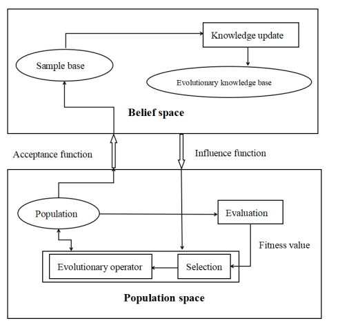
In this paper, we mainly study the equivalence and computing between Nash equilibria and the solutions to the system of equations. First, we establish a new equivalence theorem between Nash equilibria of $ n $-person noncooperative games and solutions of algebraic equations with parameters, that is, finding a Nash equilibrium point of the game is equivalent to solving a solution of the system of equations, which broadens the methods of finding Nash equilibria and builds a connection between these two types of problems. Second, an adaptive differential evolution algorithm based on cultural algorithm (ADECA) is proposed to compute the system of equations. The ADECA algorithm applies differential evolution (DE) algorithm to the population space of cultural algorithm (CA), and increases the efficiency by adaptively improving the mutation factor and crossover operator of the DE algorithm and applying new mutation operation. Then, the convergence of the ADECA algorithm is proved by using the finite state Markov chain. Finally, the new equivalence of solving Nash equilibria and the practicability and effectiveness of the algorithm proposed in this paper are verified by computing three classic games.

| [1] |
M. J. Beckmann, Spatial oligopoly as a noncooperative game, Int. J. Game Theory, 2 (1973), 263–268. https://doi.org/10.1007/BF01737575 doi: 10.1007/BF01737575

|
| [2] |
A. Muthoo, M. J. Osborne, A. Rubinstein, A course in game theory, Economica, 63 (1996), 164–165. https://doi.org/10.2307/2554642 doi: 10.2307/2554642
|
| [3] |
E. Braggion, N. Gatti, R. Lucchetti, T. Sandholm, B. von Stengel, Strong Nash equilibria and mixed strategies, Int. J. Game Theory, 49 (2020), 699–710. https://doi.org/10.1007/s00182-020-00723-3 doi: 10.1007/s00182-020-00723-3
|
| [4] | J. V. Neumann, O. Morgenstern, The theory of games and economic behaviour, Princeton: Princeton University Press, 1944. |
| [5] |
J. F. Nash, Equilibrium points in n-person games, Proc. Natl. Acad. Sci. USA, 36 (1950), 48–49. https://doi.org/10.1073/pnas.36.1.48 doi: 10.1073/pnas.36.1.48
|
| [6] |
J. F. Nash, Non-cooperative games, Ann. Math., 54 (1951), 286–295. https://doi.org/10.2307/1969529 doi: 10.2307/1969529
|
| [7] |
I. M. Bomze, Non-cooperative two-person games in biology: a classification, Int. J. Game Theory, 15 (1986), 31–57. https://doi.org/10.1007/BF01769275 doi: 10.1007/BF01769275
|
| [8] |
S. Govindan, R. Wilson, A global newton method to compute Nash equilibria, J. Econ. Theory, 110 (2003), 65–86. https://doi.org/10.1016/S0022-0531(03)00005-X doi: 10.1016/S0022-0531(03)00005-X
|
| [9] |
C. E. Lemke, J. T. Howson Jr., Equilibrium points of bimatrix games, Journal of the Society for Industrial and Applied Mathematics, 12 (1964), 413–423. https://doi.org/10.1137/0112033 doi: 10.1137/0112033
|
| [10] |
T. Kunieda, K. Nishimura, Finance and economic growth in a dynamic game, Dyn. Games Appl., 8 (2018), 588–600. https://doi.org/10.1007/s13235-018-0249-7 doi: 10.1007/s13235-018-0249-7
|
| [11] |
X. Wang, K. L. Teo, Generalized Nash equilibrium problem over a fuzzy strategy set, Fuzzy Set. Syst., 434 (2022), 172–184. https://doi.org/10.1016/j.fss.2021.06.006 doi: 10.1016/j.fss.2021.06.006
|
| [12] |
S. W. Xiang, S. Y. Xia, J. H. He, Y. L. Yang, C. W. Liu, Stability of fixed points of set-valued mappings and strategic stability of Nash equilibria, J. Nonlinear Sci. Appl., 10 (2017), 3599–3611. https://doi.org/10.22436/jnsa.010.07.20 doi: 10.22436/jnsa.010.07.20
|
| [13] |
S. W. Xiang, D. J. Zhang, R. Li, Y. L. Yang, Strongly essential set of KyFan's points and the stability of Nash equilibrium, J. Math. Anal. Appl., 459 (2018), 839–851. https://doi.org/10.1016/j.jmaa.2017.11.009 doi: 10.1016/j.jmaa.2017.11.009
|
| [14] |
J. P. Torres-Martínez, Fixed points as Nash equilibria, Fixed Point Theory Appl., 2006 (2006), 36135. https://doi.org/10.1155/FPTA/2006/36135 doi: 10.1155/FPTA/2006/36135
|
| [15] |
M. Schaefer, D. Štefankovič, Fixed points, Nash equilibria, and the existential theory of the reals, Theory Comput. Syst., 60 (2015), 172–193. https://doi.org/10.1007/s00224-015-9662-0 doi: 10.1007/s00224-015-9662-0
|
| [16] |
H. Mills, Equilibrium points in finite games, Journal of the Society for Industrial and Applied Mathematics, 8 (1960), 397–402. https://doi.org/10.1137/0108026 doi: 10.1137/0108026
|
| [17] |
N. G. Pavlidis, K. E. Parsopoulos, M. N. Vrahatis, Computing Nash equilibria through computational intelligence methods, J. Comput. Appl. Math., 175 (2005), 113–136. https://doi.org/10.1016/j.cam.2004.06.005 doi: 10.1016/j.cam.2004.06.005
|
| [18] |
A. S. Strekalovskii, R. Enkhbat, Polymatrix games and optimization problems, Autom. Remote Control, 75 (2014), 632–645. https://doi.org/10.1134/S0005117914040043 doi: 10.1134/S0005117914040043
|
| [19] | E. Rentsen, N. Tungalag, A. Gornov, A. Anikin, The curvilinear search algorithm for solving three-person game, In: Supplementary Proceedings of the 9th International Conference on Discrete Optimization and Operations Research and Scientific School (DOOR 2016), Vladivostok, Russia, September 19–23, 2016,574–583. |
| [20] |
H. M. Li, S. W. Xiang, Y. L. Yang, C. W. Liu, Differential evolution particle swarm optimization algorithm based on good point set for computing nash equilibrium of finite noncooperative game, AIMS Mathematics, 6 (2021), 1309–1323. https://doi.org/10.3934/math.2021081 doi: 10.3934/math.2021081
|
| [21] |
J. T. Howson Jr., Equilibria of polymatrix games, Manage. Sci., 18 (1972), 312–318. https://doi.org/10.1287/mnsc.18.5.312 doi: 10.1287/mnsc.18.5.312
|
| [22] | J. Y. Han, N. H. Xiu, H. D. Qi, Nonlinear complementarity theory and algorithm, (Chinese), Shanghai: Shanghai Scienceand Technology Press, 2006. |
| [23] |
Z. H. Huang, L. Qi, Formulating an n-person noncooperative game as a tensor complementarity problem, Comput. Optim. Appl., 66 (2017), 557–576. https://doi.org/10.1007/s10589-016-9872-7 doi: 10.1007/s10589-016-9872-7
|
| [24] |
C. Chen, L. Zhang, Finding nash equilibrium for a class of multi-person noncooperative games via solving tensor complementarity problem, Appl. Numer. Math., 145 (2019), 458–468. https://doi.org/10.1016/j.apnum.2019.05.013 doi: 10.1016/j.apnum.2019.05.013
|
| [25] |
F. Salehisadaghiani, L. Pavel, Distributed nash equilibrium seeking: a gossip-based algorithm, Automatica, 72 (2016), 209–216. https://doi.org/10.1016/j.automatica.2016.06.004 doi: 10.1016/j.automatica.2016.06.004
|
| [26] |
G. Chen, Y. Ming, Y. Hong, P. Yi, Distributed algorithm for $\varepsilon$-generalized Nash equilibria with uncertain coupled constraints, Automatica, 123 (2021), 109313. https://doi.org/10.1016/j.automatica.2020.109313 doi: 10.1016/j.automatica.2020.109313
|
| [27] |
Y. Zou, B. Huang, Z. Meng, W. Ren, Continuous-time distributed nash equilibrium seeking algorithms for non-cooperative constrained games, Automatica, 127 (2021), 109535. https://doi.org/10.1016/j.automatica.2021.109535 doi: 10.1016/j.automatica.2021.109535
|
| [28] |
C. Cenedese, G. Belgioioso, S. Grammatico, M. Cao, An asynchronous distributed and scalable generalized nash equilibrium seeking algorithm for strongly monotone games, Eur. J. Control, 58 (2021), 143–151. https://doi.org/10.1016/j.ejcon.2020.08.006 doi: 10.1016/j.ejcon.2020.08.006
|
| [29] | S. Liang, P. Yi, Y. Hong, Distributed Nash equilibrium seeking of a class of aggregative games, In: 2017 13th IEEE International Conference on Control & Automation (ICCA), Ohrid, Macedonia, 2017, 58–63. https://doi.org/10.1109/ICCA.2017.8003035 |
| [30] |
M. Ye, G. Hu, Distributed Nash equilibrium seeking by a consensus based approach, IEEE Trans. Automat. Contr., 62 (2017), 4811–4818. https://doi.org/10.1109/TAC.2017.2688452 doi: 10.1109/TAC.2017.2688452
|
| [31] |
X. Wang, A computational approach to dynamic generalized Nash equilibrium problem with time delay, Commun. Nonlinear Sci. Numer. Simulat., 117 (2023), 106954. https://doi.org/10.1016/j.cnsns.2022.106954 doi: 10.1016/j.cnsns.2022.106954
|
| [32] | J. Yu, Selection of game theory, (Chinese), Beijing: Science Press, 2014. |
| [33] | R. G. Reynolds, W. Sverdlik, Problem solving using cultural algorithms, In: Proceedings of the First IEEE Conference on Evolutionary Computation, IEEE World Congress on Computational Intelligence, Orlando, FL, USA, 1994,645–650. https://doi.org/10.1109/ICEC.1994.349983 |
| [34] | R. Storn, K. Price, Minimizing the real functions of the icec'96 contest by differential evolution, In: Proceedings of IEEE international conference on evolutionary computation, Nagoya, Japan, 1996,842–844. https://doi.org/10.1109/ICEC.1996.542711 |
| [35] | K. Price, P. M. Storn, J. A. Lampinen, Differential evolution: a practical approach to global optimization, Berlin, Heidelberg: Springer, 2005. https://doi.org/10.1007/3-540-31306-0 |
| [36] | N. Noman, H. Iba, Enhancing differential evolution performance with local search for high dimensional function optimization, In: Proceedings of the 7th annual conference on Genetic and evolutionary computation, 2005,967–974. https://doi.org/10.1145/1068009.1068174 |
| [37] | S. M. Saleem, Knowledge-based solution to dynamic optimization problems using cultural algorithms, PhD thesis, Wayne State University, Detroit, Michigan, 2001. |
| [38] |
Z. B. Xu, Z. P. Chen, X. S. Zhang, Theoretical development on genetic algorithms: a review, (Chinese), Advances in Mathematics, 29 (2000), 97–114. https://doi.org/10.3969/j.issn.1000-0917.2000.02.001 doi: 10.3969/j.issn.1000-0917.2000.02.001
|
| [39] | B. Zhang, J. X. Zhang, Applied stochastic processes, (Chinese), Beijing: Tsinghua University Press, 2006. |
| [40] | W. X. Zhang, Y. Liang, Mathematical foundation of geneticalgorithms, (Chinese), Xi'an: Xi'an Jiaotong University Press, 2001. |


Figures(4)

Huimin Li, Shuwen Xiang, Shunyou Xia, Shiguo Huang. Finding the Nash equilibria of $ n $-person noncooperative games via solving the system of equations[J]. AIMS Mathematics, 2023, 8(6): 13984-14007. doi: 10.3934/math.2023715


 DownLoad: