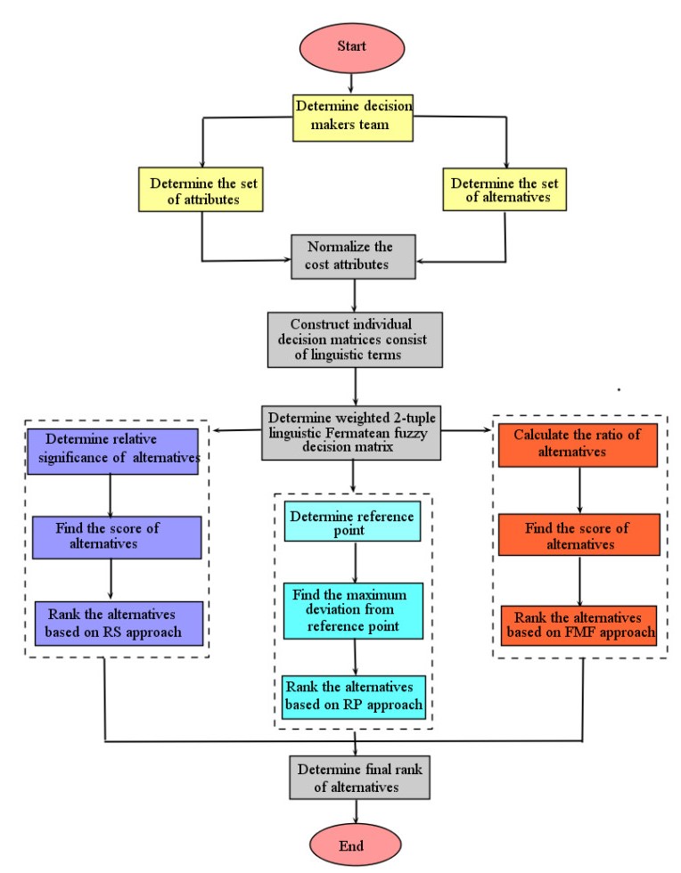
This article elaborates the enormous theory of MULTIMOORA (multi-objective optimization ratio analysis plus full multiplicative form) method to build up a new outranking approach for the innovative extension of fuzzy set theory, namely, 2-tuple linguistic Fermatean fuzzy sets (2TLFFSs). The main objective of the proposed work is to expand and present the components of MULTIMOORA method in 2-tuple linguistic Fermatean fuzzy framework. The resulted technique is named as 2-tuple linguistic Fermatean fuzzy MULTIMOORA method. This technique is designed to tackle the unclear information using 2-tuple linguistic Fermatean fuzzy numbers (2TLFFNs). The proposed model is intrinsically superior to deal with one-dimensional linguistic data. The 2TLFF-MULTIMOORA method takes into account standard relative correlations. Also, it handles the rank inversion problem when changing the rank of alternatives by adding one or more alternatives. The algorithm designed for the proposed methodology is elaborated with a numerical example (to opt for the most favorable city for the selection of quality of life). The accuracy and precision of the proposed strategy is determined by narrating a comparative study. Finally, the advantages of the developed technique over existing methods are discussed briefly.
Citation: Muhammad Akram, Naila Ramzan, Anam Luqman, Gustavo Santos-García. An integrated MULTIMOORA method with 2-tuple linguistic Fermatean fuzzy sets: Urban quality of life selection application[J]. AIMS Mathematics, 2023, 8(2): 2798-2828. doi: 10.3934/math.2023147
This article elaborates the enormous theory of MULTIMOORA (multi-objective optimization ratio analysis plus full multiplicative form) method to build up a new outranking approach for the innovative extension of fuzzy set theory, namely, 2-tuple linguistic Fermatean fuzzy sets (2TLFFSs). The main objective of the proposed work is to expand and present the components of MULTIMOORA method in 2-tuple linguistic Fermatean fuzzy framework. The resulted technique is named as 2-tuple linguistic Fermatean fuzzy MULTIMOORA method. This technique is designed to tackle the unclear information using 2-tuple linguistic Fermatean fuzzy numbers (2TLFFNs). The proposed model is intrinsically superior to deal with one-dimensional linguistic data. The 2TLFF-MULTIMOORA method takes into account standard relative correlations. Also, it handles the rank inversion problem when changing the rank of alternatives by adding one or more alternatives. The algorithm designed for the proposed methodology is elaborated with a numerical example (to opt for the most favorable city for the selection of quality of life). The accuracy and precision of the proposed strategy is determined by narrating a comparative study. Finally, the advantages of the developed technique over existing methods are discussed briefly.

| [1] | W. K. Brauers, E. K. Zavadskas, The MOORA method and its application to privatization in a transition economy, Control Cybern., 35 (2006), 445–469. |
| [2] |
W. K. M. Brauers, E. K. Zavadskas, Project management by MULTIMOORA as an instrument for transition economies, Technol. Econ. Dev. Eco., 16 (2010), 5–24. https://doi.org/10.3846/tede.2010.01 doi: 10.3846/tede.2010.01

|
| [3] | L. A. Zadeh, Fuzzy sets, Inform. Control, 8 (1965), 338–353. |
| [4] | T. Senapati, R. R. Yager, Fermatean fuzzy sets, J. Amb. Intel. Hum. Comp., 11 (2020), 663–674. https://doi.org/10.1007/s12652-019-01377-0 |
| [5] | K. T. Atanassov, Intuitionistic fuzzy sets, Int. J. Bioautom., 20 (2016), 1–6. https://doi.org/10.1016/S0165-0114(86)80034-3 |
| [6] | R. R. Yager, Pythagorean fuzzy subsets, In 2013 Joint IFSA World Congress and NAFIPS Annual Meeting (IFSA/NAFIPS), 2013, 57–61. https://doi.org/10.1109/IFSA-NAFIPS.2013.6608375 |
| [7] |
L. A. Zadeh, The concept of a linguistic variable and its application to approximate reasoning, Inform. Sci., 8 (1975), 199–249. https://doi.org/10.1016/0020-0255(75)90017-1 doi: 10.1016/0020-0255(75)90017-1
|
| [8] |
S. Chakraborty, Applications of the MOORA method for decision making in manufacturing environment, Int. J. Adv. Manuf. Tech., 54 (2011), 1155–1166. https://doi.org/10.1007/s00170-010-2972-0 doi: 10.1007/s00170-010-2972-0
|
| [9] |
P. Karande, S. Chakraborty, Application of multi-objective optimization on the basis of ratio analysis (MOORA) method for materials selection, Mater. Design, 37 (2012), 317–324. https://doi.org/10.1016/j.matdes.2012.01.013 doi: 10.1016/j.matdes.2012.01.013
|
| [10] |
W. K. M. Brauers, E. K. Zavadskas, S. Kildiene, Was the construction sector in 20 European countries anti-cyclical during the recession years 2008–2009 as measured by multicriteria analysis (MULTIMOORA), Proc. Comput. Sci., 31 (2014), 949–956. https://doi.org/10.1016/j.procs.2014.05.347 doi: 10.1016/j.procs.2014.05.347
|
| [11] |
W. K. M. Brauers, E. K. Zavadskas, MULTIMOORA optimization used to decide on a bank loan to buy property, Technol. Econ. Dev. Eco., 17 (2011), 259–290. https://doi.org/10.3846/13928619.2011.560632 doi: 10.3846/13928619.2011.560632
|
| [12] |
Z. S. Chen, X. Zhang, R. M. Rodríguez, W. Pedrycz, L. Martínez, Expertise-based bid evaluation for construction-contractor selection with generalized comparative linguistic ELECTRE III, Automat. Constr., 125 (2021), 103578. https://doi.org/10.1016/j.autcon.2021.103578 doi: 10.1016/j.autcon.2021.103578
|
| [13] |
Z. S. Chen, X. Zhang, W. Pedrycz, X. J. Wang, M. J. Skibniewski, Bid evaluation in civil construction under uncertainty: A two-stage LSP-ELECTRE III-based approach, Eng. Appl. Artrif. Intell., 94 (2020), 103835. https://doi.org/10.1016/j.engappai.2020.103835 doi: 10.1016/j.engappai.2020.103835
|
| [14] |
W. K. M. Brauers, A. Bale$\check{z}$entis, T. Bale$\check{z}$entis, MULTIMOORA for the EU Member States updated with fuzzy number theory, Technol. Econ. Dev. Eco., 17 (2011), 259–290. https://doi.org/10.3846/20294913.2011.580566 doi: 10.3846/20294913.2011.580566
|
| [15] |
A. Hafezalkotob, A. Hafezalkotob, H. Liao, F. Herrera, An overview of MULTIMOORA for multi-criteria decision-making: Theory, developments, applications, and challenges, Inform. Fusion, 51 (2019), 145–177. https://doi.org/https://doi.org/10.1016/j.inffus.2018.12.002 doi: 10.1016/j.inffus.2018.12.002
|
| [16] |
T. Bale$\check{z}$entis, A. Bale$\check{z}$entis, A survey on development and applications of the multi-criteria decision making method MULTIMOORA, J. Multi-Criteria Dec., 21 (2014), 209–222. https://doi.org/https://doi.org/10.1002/mcda.1501 doi: 10.1002/mcda.1501
|
| [17] |
Ö. Alkan, Ö. K. Albayrak, Ranking of renewable energy sources for regions in Turkey by fuzzy entropy based fuzzy COPRAS and fuzzy MULTIMOORA, Renew. Energy, 162 (2020), 712–726. https://doi.org/10.1016/j.renene.2020.08.062 doi: 10.1016/j.renene.2020.08.062
|
| [18] |
W. Liang, G. Zhao, C. Hong, Selecting the optimal mining method with extended multi-objective optimization by ratio analysis plus the full multiplicative form (MULTIMOORA) approach, Neural Comput. Appl., 31 (2019), 5871–5886. https://doi.org/10.1007/s00521-018-3405-5 doi: 10.1007/s00521-018-3405-5
|
| [19] |
H. C. Liu, X. J. Fan, P. Li, Y. Z. Chen, Evaluating the risk of failure modes with extended MULTIMOORA method under fuzzy environment, Eng. Appl. Artif. Intell., 34 (2014), 168–177. https://doi.org/10.1016/j.engappai.2014.04.011 doi: 10.1016/j.engappai.2014.04.011
|
| [20] |
R. Fattahi, M. Khalilzadeh, Risk evaluation using a novel hybrid method based on FMEA, extended MULTIMOORA, and AHP methods under fuzzy environment, Safety Sci., 102 (2018), 290–300. https://doi.org/https://doi.org/10.1016/j.ssci.2017.10.018 doi: 10.1016/j.ssci.2017.10.018
|
| [21] |
J. H. Dahooie, E. K. Zavadskas, H. R. Firoozfar, A. S. Vanaki, N. Mohammadi, W. K. M. Brauers, An improved fuzzy MULTIMOORA approach for multi-criteria decision making based on objective weighting method (CCSD) and its application to technological forecasting method selection, Eng. Appl. Artif. Intell., 79 (2018), 114–128. https://doi.org/10.1016/j.engappai.2018.12.008 doi: 10.1016/j.engappai.2018.12.008
|
| [22] |
Z. S. Chen, Y. Yang, X. J. Wang, K. S. Chin, K. L. Tsui, Fostering linguistic decision-making under uncertainty: A proportional interval type-2 hesitant fuzzy TOPSIS approach based on Hamacher aggregation operators and andness optimization models, Inform. Sci., 500 (2019), 229–258. https://doi.org/10.1016/j.ins.2019.05.074 doi: 10.1016/j.ins.2019.05.074
|
| [23] |
C. Zhang, C. Chen, D. Streimikiene, T. Balezentis, Intuitionistic fuzzy MULTIMOORA approach for multi-criteria assessment of the energy storage technologies, Appl. Soft Comput., 79 (2019), 410–423. https://doi.org/10.1016/j.asoc.2019.04.008 doi: 10.1016/j.asoc.2019.04.008
|
| [24] |
H. Garg, D. Rani, An efficient intuitionistic fuzzy MULTIMOORA approach based on novel aggregation operators for the assessment of solid waste management techniques, Appl. Intell., 52 (2021), 1–34. https://doi.org/10.1007/s10489-021-02541-w doi: 10.1007/s10489-021-02541-w
|
| [25] |
C. Huang, M. Lin, Z. Xu, Pythagorean fuzzy MULTIMOORA method based on distance measure and score function: Its application in multicriteria decision making process, Knowl. Inform. Syst., 62 (2020), 4373–4406. https://doi.org/10.1007/s10115-020-01491-y doi: 10.1007/s10115-020-01491-y
|
| [26] |
X. H. Li, L. Huang, Q. Li, H. C. Liu, Passenger satisfaction evaluation of public transportation using Pythagorean fuzzy MULTIMOORA method under large group environment, Sustainability, 12 (2020), 4996. https://doi.org/10.3390/su12124996 doi: 10.3390/su12124996
|
| [27] |
T. Senapati, R. R. Yager, Some new operations over Fermatean fuzzy numbers and application of Fermatean fuzzy WPM in multiple criteria decision making, Informatica, 2 (2019), 391–412. https://doi.org/10.15388/Informatica.2019.211 doi: 10.15388/Informatica.2019.211
|
| [28] |
T. Senapati, R. R. Yager, Fermatean fuzzy weighted averaging/geometric operators and its application in multi-criteria decision-making methods, Eng. Appl. Artrif. Intel., 85 (2019), 112–121. https://doi.org/10.1016/j.engappai.2019.05.012 doi: 10.1016/j.engappai.2019.05.012
|
| [29] | H. Garg, G. Shahzadi, M. Akram, Decision-making analysis based on Fermatean fuzzy Yager aggregation operators with application in COVID-19 testing facility, Math. Probl. Eng., 2020 (2020). https://doi.org/10.1155/2020/7279027 |
| [30] |
P. Rani, A. R. Mishra, Fermatean fuzzy Einstein aggregation operators-based MULTIMOORA method for electric vehicle charging station selection, Expert Syst. Appl., 182 (2021), 115267. https://doi.org/10.1016/j.eswa.2021.115267 doi: 10.1016/j.eswa.2021.115267
|
| [31] |
X. Chen, L. Zhao, H. Liang, A novel multi-attribute group decision-making method based on the MULTIMOORA with linguistic evaluations, Soft Comput., 22 (2018), 5347–5361. https://doi.org/10.1007/s00500-018-3030-3 doi: 10.1007/s00500-018-3030-3
|
| [32] |
H. Zhang, Linguistic intuitionistic fuzzy sets and application in MAGDM, J. Appl. Math., 2014 (2014), 1–11. https://doi.org/10.1155/2014/432092 doi: 10.1155/2014/432092
|
| [33] |
Z. Chen, P. Liu, Z. Pei, An approach to multiple attribute group decision making based on linguistic intuitionistic fuzzy numbers, Int. J. Comput. Intell., 8 (2015), 747–760. https://doi.org/10.1080/18756891.2015.1061394 doi: 10.1080/18756891.2015.1061394
|
| [34] |
H. Garg, Linguistic Pythagorean fuzzy sets and its applications in multiattribute decision-making process, Int. J. Comput. Intell., 33 (2018), 1234–1263. https://doi.org/10.1002/int.21979 doi: 10.1002/int.21979
|
| [35] | M. Akram, N. Ramzan, F. Feng, Extending COPRAS method with linguistic Fermatean fuzzy sets and Hamy mean operators, J. Math., 2022 (2022). https://doi.org/10.1155/2022/8239263 |
| [36] |
M. Akram, S. Naz, S. A. Edalatpanah, R. Mehreen, Group decision-making framework under linguistic $q$-rung orthopair fuzzy Einstein models, Soft Comput., 25 (2021), 10309–10334. https://doi.org/10.1007/s00500-021-05771-9 doi: 10.1007/s00500-021-05771-9
|
| [37] |
P. Liu, S. Naz, M. Akram, M. Muzammal, Group decision-making analysis based on linguistic $q$-rung orthopair fuzzy generalized point weighted aggregation operators, Int. J. Mach. Learn. Cyb., 13 (2022), 883–906. https://doi.org/10.1007/s13042-021-01425-2 doi: 10.1007/s13042-021-01425-2
|
| [38] |
T. Mahmood, M. S. Warraich, Z. Ali, D. Pamucar, Generalized MULTIMOORA method and Dombi prioritized weighted aggregation operators based on T-spherical fuzzy sets and their applications, Int.J. Intell. Syst., 36 (2021), 4659–4692. https://doi.org/10.1002/int.22474 doi: 10.1002/int.22474
|
| [39] |
S. Naz, M. Akram, A. B. Saeid, A. Saadat, Models for MAGDM with dual hesitant $q$-rung orthopair fuzzy 2-tuple linguistic MSM operators and their application to COVID-19 pandemic, Expert Syst., 39 (2022), e13005. https://doi.org/10.1111/exsy.13005 doi: 10.1111/exsy.13005
|
| [40] |
S. Xian, Z. Liu, X. Gou, W. Wan, Interval 2-tuple Pythagorean fuzzy linguistic MULTIMOORA method with CIA and their application to MCGDM, Int. J. Intell. Syst., 35 (2020), 650–681. https://doi.org/10.1002/int.22221 doi: 10.1002/int.22221
|
| [41] |
M. Akram, F. Ilyas, H. Garg, ELECTRE-II method for group decision-making in Pythagorean fuzzy environment, Appl. Intell., 51 (2021), 8701–8719. https://doi.org/10.1007/s10489-021-02200-0 doi: 10.1007/s10489-021-02200-0
|
| [42] | M. Akram, U. Noreen, M. M. Ali Al-Shamiri, Decision analysis approach based on 2-tuple linguistic-polar fuzzy Hamacher aggregation operators, Discrete Dyn. Nat. Soc., 2022 (2022). https://doi.org/10.1155/2022/6269115 |
| [43] | S. Naz, M. Akram, G. Muhiuddin, A. Shafiq, Modified EDAS method for MAGDM based on MSM operators with 2-tuple linguistic-spherical fuzzy sets, Math. Probl. Eng., 2022 (2022). https://doi.org/10.1155/2022/5075998 |
| [44] |
G. Kou, H. Xiao, M. Cao, L. H. Lee, Optimal computing budget allocation for the vector evaluated genetic algorithm in multi-objective simulation optimization, Automatica, 129 (2021), 109599. https://doi.org/10.1016/j.automatica.2021.109599 doi: 10.1016/j.automatica.2021.109599
|
| [45] |
G. Kou, Ö. Olgu Akdeniz, H. Dinçer, S. Yüksel, Fintech investments in European banks: A hybrid IT2 fuzzy multidimensional decision-making approach, Financ. Innov., 7 (2021), 1–28. https://doi.org/10.1186/s40854-021-00256-y doi: 10.1186/s40854-021-00256-y
|
| [46] |
G. Li, G. Kou, Y. Li, Y. Peng, A group decision making approach for supplier selection with multi-period fuzzy information and opinion interaction among decision makers, J. Oper. Res. Soc., 73 (2022), 855–868. https://doi.org/10.1080/01605682.2020.1869917 doi: 10.1080/01605682.2020.1869917
|
| [47] | X. Ding, J. Zhong, Power battery recycling mode selection using an extended MULTIMOORA method, Sci. Programming, 2018 (2018). https://doi.org/10.1155/2018/7675094 |
| [48] |
L. Martínez, F. Herrera, An overview on the 2-tuple linguistic model for computing with words in decision making: Extensions, applications and challenges, Inform. Sci., 207 (2012), 1–18. https://doi.org/10.1016/j.ins.2012.04.025 doi: 10.1016/j.ins.2012.04.025
|
| [49] |
F. Herrera, L. Martínez, A 2-tuple fuzzy linguistic representation model for computing with words, IEEE T. Fuzzy Syst., 8 (2000), 746–752. https://doi.org/10.1109/91.890332 doi: 10.1109/91.890332
|
| [50] | L. Martínez, R. M. Rodriguez, F. Herrera, 2-Tuple linguistic model, In the 2-Tuple Linguistic Model, Springer, Cham, 392 (2015), 23–42. https://doi.org/10.1007/978-3-319-24714-4_2 |
| [51] | A. Bale$\check{z}$entis, T. Bale$\check{z}$entis, An innovative multi-criteria supplier selection based on two-tuple MULTIMOORA and hybrid data, Econ. Comput. Econ. Cyb., 45 (2011), 37–56. |
| [52] |
G. W. Wei, 2-tuple intuitionistic fuzzy linguistic aggregation operators in multiple attribute decision making, Iran. J. Fuzzy Syst., 16 (2019), 159–174. https://doi.org/10.22111/IJFS.2019.4789 doi: 10.22111/IJFS.2019.4789
|
| [53] |
X. Deng, J. Wang, G. Wei, M. Lu, Models for multiple attribute decision making with some 2-tuple linguistic Pythagorean fuzzy Hamy mean operators, Mathematics, 6 (2018), 236. https://doi.org/10.3390/math6110236 doi: 10.3390/math6110236
|
| [54] |
X. Deng, J. Wang, G. Wei, Some 2-tuple linguistic Pythagorean Heronian mean operators and their application to multiple attribute decision-making, J. Exp. Theor. Artif. Intell., 31 (2019), 555–574. https://doi.org/10.1080/0952813X.2019.1579258 doi: 10.1080/0952813X.2019.1579258
|
| [55] | M. Akram, A. Khan, U. Ahmad, Extended MULTIMOORA method based on 2-tuple linguistic Pythagorean fuzzy sets for multi-attribute group decision-making, Granular Comput., 2022. https://doi.org/10.1007/s41066-022-00330-5 |
| [56] |
X. Deng, H. Gao, TODIM method for multiple attribute decision making with 2-tuple linguistic Pythagorean fuzzy information, J. Intell. Fuzzy Syst., 37 (2019), 1769–1780. https://doi.org/10.3233/JIFS-179240 doi: 10.3233/JIFS-179240
|
| [57] | M. Akram, R. Bibi, M. A. Al-Shamiri, A decision-making framework based on 2-tuple linguistic Fermatean fuzzy Hamy mean operators, Math. Probl. Eng., 2022 (2022). https://doi.org/10.1155/2022/1501880 |
| [58] |
Q. Y. Chen, H. C. Liu, J. H. Wang, H. Shi, New model for occupational health and safety risk assessment based on Fermatean fuzzy linguistic sets and CoCoSo approach, Appl. Soft Comput., 126 (2022), 109262. https://doi.org/10.1016/j.asoc.2022.109262 doi: 10.1016/j.asoc.2022.109262
|
| [59] |
S. M. Wu, X. Y. You, H. C. Liu, L. E. Wang, Improving quality function deployment analysis with the cloud MULTIMOORA method, Int. T. Oper. Res., 27 (2020), 1600–1621. https://doi.org/10.1111/itor.12484 doi: 10.1111/itor.12484
|
| [60] |
Z. S. Chen, K. S. Chin, Y. L. Li, Y. Yang, On generalized extended Bonferroni means for decision making, IEEE T. Fuzzy Syst., 24 (2016), 1525–1543. https://doi.org/10.1109/TFUZZ.2016.2540066 doi: 10.1109/TFUZZ.2016.2540066
|
| [61] |
S. H. Xiong, Z. S. Chen, J. P. Chang, K. S. Chin, On extended power average operators for decision-making: A case study in emergency response plan selection of civil aviation, Comput. Ind. Eng., 130 (2019), 258–271. https://doi.org/10.1016/j.cie.2019.02.027 doi: 10.1016/j.cie.2019.02.027
|
| [62] |
G. Li, Q. Weng, Measuring the quality of life in city of Indianapolis by integration of remote sensing and census data, Int. J. Remote Sens., 28 (2007), 249–267. https://doi.org/10.1080/01431160600735624 doi: 10.1080/01431160600735624
|
| [63] | M. Stathopoulou, C. Cartalis, Mapping quality of life in metropolitan Athens using satellite and census data, 1st EARSEL Workshop of the SIG Urban Remote Sensing, Humboldt University, Berlín, 2–3 (2006). |
| [64] | H. Azizi, M. Momeni, M. Taghinia, Quality of life indices assessment for disabled and elderly people: Case study of Tehran, In Proceedings of the 16th International Conference on Urban Planning, Regional Development and Information Society, North Rhine-Westphalia, Germany, 2011. Available from: https://programm.corp.at/cdrom2011/papers2011/CORP2011_96.pdf. |
Figures(8) / Tables(19)

Muhammad Akram, Naila Ramzan, Anam Luqman, Gustavo Santos-García. An integrated MULTIMOORA method with 2-tuple linguistic Fermatean fuzzy sets: Urban quality of life selection application[J]. AIMS Mathematics, 2023, 8(2): 2798-2828. doi: 10.3934/math.2023147


 DownLoad: