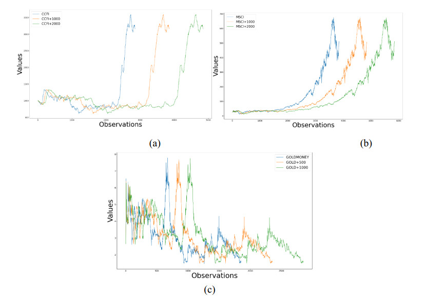
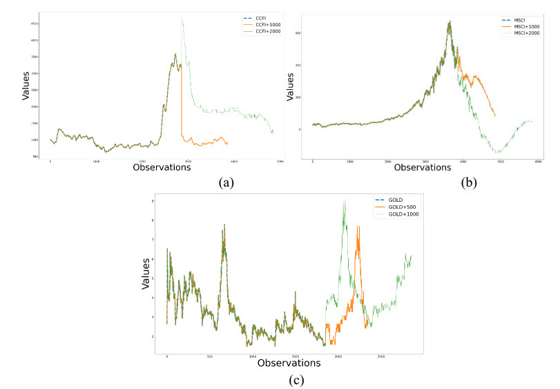
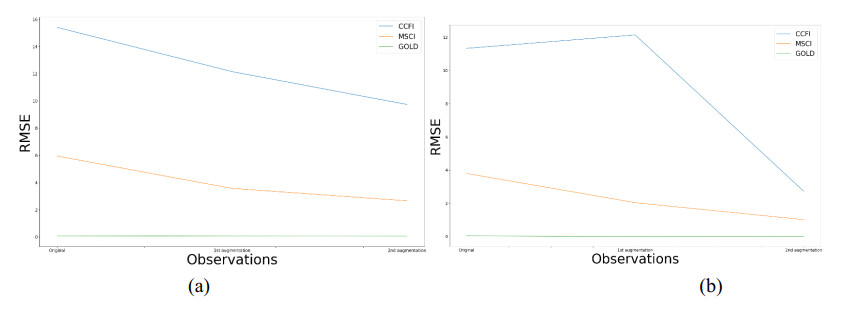
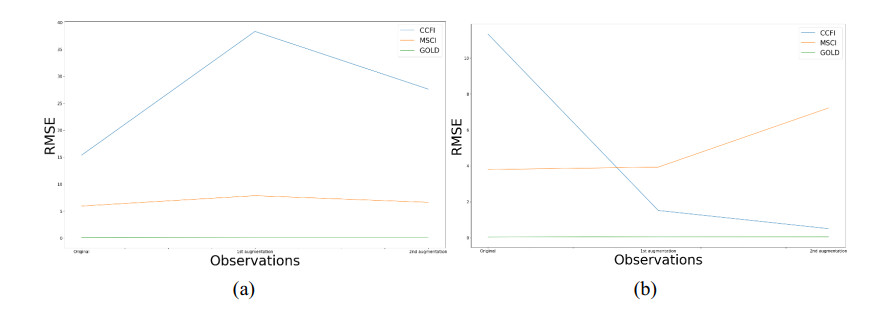
The performance of neural networks and statistical models in time series prediction is conditioned by the amount of data available. The lack of observations is one of the main factors influencing the representativeness of the underlying patterns and trends. Using data augmentation techniques based on classical statistical techniques and neural networks, it is possible to generate additional observations and improve the accuracy of the predictions. The particular characteristics of economic time series make it necessary that data augmentation techniques do not significantly influence these characteristics, this fact would alter the quality of the details in the study. This paper analyzes the performance obtained by two data augmentation techniques applied to a time series and finally processed by an ARIMA model and a neural network model to make predictions. The results show a significant improvement in the predictions by the time series augmented by traditional interpolation techniques, obtaining a better fit and correlation with the original series.
Citation: Ana Lazcano de Rojas. Data augmentation in economic time series: Behavior and improvements in predictions[J]. AIMS Mathematics, 2023, 8(10): 24528-24544. doi: 10.3934/math.20231251
The performance of neural networks and statistical models in time series prediction is conditioned by the amount of data available. The lack of observations is one of the main factors influencing the representativeness of the underlying patterns and trends. Using data augmentation techniques based on classical statistical techniques and neural networks, it is possible to generate additional observations and improve the accuracy of the predictions. The particular characteristics of economic time series make it necessary that data augmentation techniques do not significantly influence these characteristics, this fact would alter the quality of the details in the study. This paper analyzes the performance obtained by two data augmentation techniques applied to a time series and finally processed by an ARIMA model and a neural network model to make predictions. The results show a significant improvement in the predictions by the time series augmented by traditional interpolation techniques, obtaining a better fit and correlation with the original series.

| [1] | G. E. Box, G. M. Jenkins, G. C. Reinsel, Time series analysis: Forecasting and control, Holden-Day, 1970. |
| [2] | R. H. Shumway, D. S. Stoffer, Time series analysis and its applications: with R examples. Springer, 2017. https://doi.org/10.1007/978-3-319-52452-8_3 |
| [3] |
B. K. Iwana, S. Uchida, An empirical survey of data augmentation for time series classification with neural networks, PLoS ONE 16 (2021), 0254841. https://doi.org/10.1371/journal.pone.0254841 doi: 10.1371/journal.pone.0254841

|
| [4] |
G. Iglesias, E. Talavera, Á. González-Prieto, A. Mozo, S. Gómez-Canaval, Data Augmentation techniques in time series domain: a survey and taxonomy, Neural Comput. Appl., 35 (2023), 10123–10145. https://doi.org/10.1007/s00521-023-08459-3 doi: 10.1007/s00521-023-08459-3
|
| [5] | B. Liu, Z. Zhang, R. Cui, Efficient time series augmentation methods, In: 2020 13th international congress on image and signal processing, Bio. Med. Eng. Inf., 2020, 1004–1009. https://doi.org/10.1109/cisp-bmei51763.2020.9263602 |
| [6] | Y. Cheng, D. M. Titterington, Neural networks: A review from a statistical perspective, Stat. Sci., 9 (1994), 2–45. http://www.jstor.org/stable/2246275. |
| [7] |
S. H. Kim, I. Han, Genetic algorithms approach to feature discretization in artificial neural networks for the prediction of stock price index, Expert Syst. Appl., 19 (2000), 125–132. https://doi.org/10.1016/S0957-4174(00)00027-0 doi: 10.1016/S0957-4174(00)00027-0
|
| [8] | S. Lahmiri, Modeling Stock Market Industrial Sectors as Dynamic Systems and Forecasting, In: Encyclopedia of Information Science and Technology, Third Edition, IGI Global, 2015, 3818–3830. https://doi.org/10.4018/978-1-4666-5888-2.ch376 |
| [9] |
Y. Lecun, L. Bottou, Y. Bengio, P. Haffner, Gradient-based learning applied to document recognition, P. IEEE, 86 (1998), 2278–2324. https://doi.org/10.1109/5.726791 doi: 10.1109/5.726791
|
| [10] | P. Y. Simard, D. Steinkraus, J. C. Platt, Best practices for convolutional neural networks applied to visual document analysis, In: Icdarm 3 (2003), No. 2003. https://doi.org/10.1109/icdar.2003.1227801 |
| [11] | X. Glorot, A. Bordes, Y. Bengio, Deep sparse rectifier neural networks, In: Proceedings of the fourteenth international conference on artificial intelligence and statistics, JMLR Workshop and Conference Proceedings, 2011,315–323. |
| [12] | M. Daoust, J.Bégin, C. Gagné, Data augmentation using conditional generative adversarial networks for the detection of cyberbullying, In: Proceedings of the 2016 IEEE/ACM International Conference on Advances in Social Networks Analysis and Mining, IEEE, 2016,615–618. https://doi.org/10.1109/asonam.2016.7752342 |
| [13] | A. Wong, C. Leung, A review on data augmentation techniques for deep learning, In: Proceedings of the 31st International Conference on Neural Information Processing Systems, 2018, 2234–2244. |
| [14] |
H. Yao, S. Zhao, Z. Gao, Z. Xue, B. Song, F. Li, et al., Data-driven analysis on the subbase strain prediction: A deep data augmentation-based study, Transp. Geotech., 40 (2023), 100957. https://doi.org/10.1016/j.trgeo.2023.100957 doi: 10.1016/j.trgeo.2023.100957
|
| [15] | J. Yoon, J. Jordon, M. van der Schaar, TimeGAN: Preprocessing raw data for time series generation with generative adversarial networks, Proceedings of the 36th International Conference on Machine Learning, 48 (2019), 7272–7281. |
| [16] |
A. Rasheed, O. San, T. Kvamsdal, Digital twin: Values, challenges and enablers from a modeling perspective, Ieee Access, 8 (2020), 21980–22012. https://doi.org/10.1109/access.2020.2970143 doi: 10.1109/access.2020.2970143
|
| [17] | J. Jeon, J. Kim, H. Song, S. Cho, N. Park, GT-GAN: General purpose time series synthesis with generative adversarial networks, Adv. Neural Inf. Process. Syst., 35 (2022), 36999–37010. |
| [18] |
P., Chlap, H. Min, N. Vandenberg, J. Dowling, L. Holloway, A. Haworth, A review of medical image data augmentation techniques for deep learning applications, J. Med. Imag. Radiat. On., 65 (2021), 545–563. https://doi.org/10.1111/1754-9485.13261 doi: 10.1111/1754-9485.13261
|
| [19] | H. Naveed, Survey: image mixing and deleting for data augmentation, arXiv preprint arXiv: 2106.07085, 2021. https://doi.org/10.48550/arXiv.2106.07085 |
| [20] | S. Y. Feng, V. Gangal, J. Wei, S. Chandar, S. Vosoughi, T. Mitamura, et al., A survey of data augmentation approaches for nlp, arXiv preprint arXiv: 2105.03075, 2021. https://doi.org/10.18653/v1/2021.findings-acl.84 |
| [21] | Q. Wen, L. Sun, F. Yang, X. Song, J. Gao, X. Wang, et al., Time series data augmentation for deep learning: A survey. arXiv preprint arXiv: 2002.12478, 2020. https://doi.org/10.48550/arXiv.2002.12478 |
| [22] |
G. García-Molina, E. Gómez-Sánchez, A. García-Sánchez, Data Augmentation by Imputation Techniques in Time Series: Application to the Spanish Electricity Market, Processes, 7 (2021), 958. https://doi.org/10.3390/pr7120958. doi: 10.3390/pr7120958
|
| [23] | A. Le Guennec, S. Malinowski, R. Tavenard, Data augmentation for time series classification using convolutional neural networks, In: ECML/PKDD workshop on advanced analytics and learning on temporal data, 2016. https://doi.org/10.1007/978-3-030-91445-5 |
| [24] | D. Salinas, S. Mehrotra, S. Mohan, DeepAR: Probabilistic forecasting with autoregressive recurrent networks, arXiv preprint arXiv: 1704.04110, 2020. https://doi.org/10.1016/j.ijforecast.2019.07.001 |
| [25] | M. S. Gashler, S. C. Ashmore, Training deep fourier neural networks to fit time-series data. In: Intelligent Computing in Bioinformatics: 10th International Conference, ICIC 2014, Taiyuan, China, August 3–6, 2014, Proceedings 10 (2014), 48–55. Springer International Publishing. https://doi.org/10.1007/978-3-319-09330-7_7 |
| [26] | H. Kim, J. Kim, S. Oh, Time series prediction with Monte Carlo tree search and online learning. In 2017 IEEE International Conference on Big Data (Big Data), 2017, 3495–3500. https://doi.org/10.1109/bigdata47090.2019.9006276 |
| [27] |
Gao, C., Zhang, N., Li, Y., Bian, F., & Wan, H.. Self-attention-based time-variant neural networks for multi-step time series forecasting. Neural Computing and Applications, 34(11) (2022), 8737-8754. https://doi.org/10.1007/s00521-021-06871-1 doi: 10.1007/s00521-021-06871-1
|
| [28] | Li, Z., Ma, C., Shi, X., Zhang, D., Li, W., & Wu, L. Tsa-gan: A robust generative adversarial networks for time series augmentation. In 2021 International Joint Conference on Neural Networks (IJCNN) 2021, 1–8. https://doi.org/10.1109/IJCNN52387.2021.9534001 |
| [29] |
X., Tan, X. Sun, W. Chen, B. Du, J. Ye, L. Sun, Investigation on the data augmentation using machine learning algorithms in structural health monitoring information, Struct. Health Monit., 20 (2021), 2054–2068. https://doi.org/10.1177/1475921721996238 doi: 10.1177/1475921721996238
|
| [30] | D. P. Kingma, M. Welling, Auto-encoding variational bayes, arXiv preprint arXiv: 1312.6114. 2013. https://doi.org/10.48550/arXiv.1312.6114 |
| [31] |
L. Deng, Deep learning: from speech recognition to language and multimodal processing, APSIPA Trans. Signal, 5 (2016). https://doi.org/10.1017/ATSIP.2015.22 doi: 10.1017/ATSIP.2015.22
|
| [32] | I. Goodfellow, Y. Bengio, A. Courville, Deep learning, MIT press, 2016. |
| [33] | P. Isola, J. Y. Zhu, T. Zhou, A. A. Efros, Image-to-image translation with conditional adversarial networks, In Proceedings of the IEEE conference on computer vision and pattern recognition, 2017, 1125–1134. https://doi.org/10.1109/cvpr.2017.632 |
| [34] |
J. Cheng, Y. Yang, X. Tang, N. Xiong, Y. Zhang, F. Lei, Generative Adversarial Networks: A Literature Review, KSⅡ T. Internet Inf., 14 (2020), 4625–4647. https://doi.org/10.3837/tiis.2020.12.001 doi: 10.3837/tiis.2020.12.001
|
| [35] |
S. Hochreiter, J. Schmidhuber, Long short-term memory, Neural Comput., 9 (1997), 1735–1780. https://doi.org/10.1162/neco.1997.9.8.1735 doi: 10.1162/neco.1997.9.8.1735
|
| [36] | A. Oord, S. Dieleman, H. Zen, K. Simonyan, O. Vinyals, A. Graves, et al., A generative model for raw audio. arXiv preprint arXiv: 1609.03499, 2016. https://doi.org/10.48550/arXiv.1609.03499 |
| [37] | L. Dinh, J. Sohl-Dickstein, S. Bengio, Density estimation using Real NVP. arXiv preprint arXiv: 1605.08803, 2014. https://doi.org/10.48550/arXiv.1605.08803 |
| [38] |
S. Suradhaniwar, S. Kar, S. S. Durbha, A. Jagarlapudi, Time series forecasting of univariate agrometeorological data: a comparative performance evaluation via one-step and multi-step ahead forecasting strategies, Sensors, 21 (2021), 2430. https://doi.org/10.3390/s21072430 doi: 10.3390/s21072430
|
| [39] |
J. H. Poynting, A comparison of the fluctuations in the price of wheat and in cotton and silk imports into Great Britain, J. Roy. Stat. Soc., 47 (1884), 34–74. https://doi.org/10.2307/2979211 doi: 10.2307/2979211
|
| [40] | R. H. Hooker, Correlation of the marriage-rate with trade, J. Roy. Stat. Soc., 64 (1901), 485–492. |
| [41] |
J. Spencer, On the graduation of the rates of sickness and mortality presented by the experience of the Manchester Unity of Oddfellows during the period 1893–97, J. Institute Actuaries, 38 (1904), 334–343. https://doi.org/10.1017/s0020268100008076 doi: 10.1017/s0020268100008076
|
| [42] | R. G. Brown, Smoothing, forecasting and prediction of discrete time series, Prentice-Hall, 1963. |
| [43] |
D. E. Rumelhart, G. E. Hinton, R. J. Williams, Learning representations by back-propagating errors, Nature, 323 (1986), 533–536. https://doi.org/10.1038/323533a0 doi: 10.1038/323533a0
|
| [44] |
G. Zhang, B. E. Patuwo, M. Y. Hu, Forecasting with artificial neural networks: The state of the art, Int. J. Forecasting, 14 (1998), 35–62. https://doi.org/10.1016/S0169-2070(97)00044-7 doi: 10.1016/S0169-2070(97)00044-7
|
| [45] |
K. Hornik, M. Stinchcombe, H. White, Multilayer feedforward networks are universal approximators, Neural Network., 2 (1989), 359–366. https://doi.org/10.1016/0893-6080(89)90020-8 doi: 10.1016/0893-6080(89)90020-8
|
| [46] |
P. J. Werbos, Generalization of backpropagation with application to a recurrent gas market model, Neural Network., 1 (1988), 339–356. https://doi.org/10.1016/0893-6080(88)90007-x doi: 10.1016/0893-6080(88)90007-x
|
| [47] |
T. Hill, M. O'Connor, W. Remus, Neural network models for time series forecasts, Manag. Sci., 42 (1996), 1082–1092. https://doi.org/10.1287/mnsc.42.7.1082 doi: 10.1287/mnsc.42.7.1082
|
| [48] | S. Siami-Namini, A. S. Namin, Forecasting economics and financial time series: ARIMA vs. LSTM. arXiv preprint arXiv: 1803.06386, 2018. https://doi.org/10.1109/icmla.2018.00227 |
| [49] |
V. Ravi, D. Pradeepkumar, K. Deb, Financial time series prediction using hybrids of chaos theory, multi-layer perceptron and multi-objective evolutionary algorithms, Swarm Evol. Comput., 36 (2017), 136–149. https://doi.org/10.1016/j.swevo.2017.05.003 doi: 10.1016/j.swevo.2017.05.003
|
| [50] |
A. Zameer, A. Khan, S. G. Javed, Machine learning based short term wind power prediction using a hybrid learning model, Comput, Electr, Eng, , 45 (2015), 122–133. https://doi.org/10.1016/j.compeleceng.2014.07.009 doi: 10.1016/j.compeleceng.2014.07.009
|
| [51] | M. Jiang, L. Jia, Z. Chen, W. Chen, The two-stage machine learning ensemble models for stock price prediction by combining mode decomposition, extreme learning machine and improved harmony search algorithm, Ann. Oper. Res., 309 (2022), 533–585. |
| [52] |
P. Du, J. Wang, W. Yang, T. Niu, A novel hybrid model for short-term wind power forecasting, Appl. Soft Comput., 80 (2019), 93–106. https://doi.org/10.1016/j.asoc.2019.03.035 doi: 10.1016/j.asoc.2019.03.035
|
| [53] |
A. Lazcano, P. J. Herrera, M. A. Monge, Combined model based on recurrent neural networks and graph convolutional networks for financial time series forecasting, Mathematics, 11 (2023), 224. https://doi.org/10.3390/math11010224 doi: 10.3390/math11010224
|
| [54] |
S. X. Lv, L. Wang, Multivariate wind speed forecasting based on multi-objective feature selection approach and hybrid deep learning model, Energy, 263 (2023), 126100. https://doi.org/10.1016/j.energy.2022.126100 doi: 10.1016/j.energy.2022.126100
|
| [55] |
F. Wang, Z. Zhang, C. Liu, Y. Yu, S. Pang, N. Duić, et al., Generative adversarial networks and convolutional neural networks based weather classification model for day ahead short-term photovoltaic power forecasting, Energ. Convers. Manage., 181 (2019), 443–462. https://doi.org/10.1016/j.enconman.2018.11.074 doi: 10.1016/j.enconman.2018.11.074
|
| [56] |
K. M. Rashid, J. Louis, Times-series data augmentation and deep learning for construction equipment activity recognition, Adv. Eng. Inform., 42 (2019), 100944. https://doi.org/10.1016/j.aei.2019.100944 doi: 10.1016/j.aei.2019.100944
|
| [57] | Y. Luo, X. Cai, Y. Zhang, J. Xu, Multivariate time series imputation with generative adversarial networks, Adv. Neural Inform. Proces. Syst., 31 (2018). |
| [58] | Q. Wen, L. Sun, F. Yang, X. Song, J. Gao, X. Wang, et al., Time series data augmentation for deep learning: A survey, arXiv preprint arXiv: 2002.12478, 2020. https://doi.org/10.48550/arXiv.2002.12478 |
| [59] |
C. Shorten, T. M. Khoshgoftaar, A survey on image data augmentation for deep learning, J. Big Data, 6 (2019), 1–48. https://doi.org/10.1186/s40537-019-0197-0 doi: 10.1186/s40537-019-0197-0
|
| [60] |
P. H. Hsieh, P. H. Liao, A comparative study of stock price forecasting models, J. Appl. Math., 111 (2019). https://doi.org/10.1155/2019/8681410 doi: 10.1155/2019/8681410
|
| [61] |
T. C.Tung, S. H.Yen, T. Y. Huang, C. P.Chen, Short-Term electric load forecasting using stacked extreme learning machine with clustering technique, Energies, 13 (2020), 3977. https://doi.org/10.3390/en13153977 doi: 10.3390/en13153977
|
| [62] |
K. Bandara, H. Hewamalage, Y. H. Liu, Y. Kang, C. Bergmeir, Improving the accuracy of global forecasting models using time series data augmentation, Pattern Recogn., 120 (2021), 108148. https://doi.org/10.1016/j.patcog.2021.108148 doi: 10.1016/j.patcog.2021.108148
|
| [63] | M. F. Asem, M. M. Abogameel, N. Almujally, A. H. Alkashan, Comparative study of interpolation methods for time series data augmentation, Proceedings of the 2021 International Conference on High Performance Computing & Simulation, 2021,110–115. |
Figures(4) / Tables(5)

Ana Lazcano de Rojas. Data augmentation in economic time series: Behavior and improvements in predictions[J]. AIMS Mathematics, 2023, 8(10): 24528-24544. doi: 10.3934/math.20231251


 DownLoad: