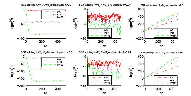
Stability for discrete time waveform relaxation methods based on Euler schemes

Junjiang Lai; Zhencheng Fan; Junjiang Lai; Zhencheng Fan

doi:10.3934/math.20231206

AIMS Mathematics

2023, Volume 8, Issue 10: 23713-23733. doi: 10.3934/math.20231206

Previous Article Next Article

Research article Special Issues

Stability for discrete time waveform relaxation methods based on Euler schemes

Junjiang Lai ,
Zhencheng Fan ^,

College of Mathematics and Data Science, Minjiang University, Fuzhou 350108, China

Received: 29 June 2023 Revised: 19 July 2023 Accepted: 19 July 2023 Published: 02 August 2023
MSC : 34D20, 65L05, 65L20

Stability properties of discrete time waveform relaxation (DWR) methods based on Euler schemes are analyzed by applying them to two dissipative systems. Some sufficient conditions for stability of the considered methods are obtained; at the same time two examples of instability are given. To investigate the influence of the splitting functions and underlying numerical methods on stability of DWR methods, DWR methods based on different splittings and different numerical schemes are considered. The obtained results show that the stabilities of waveform relaxation methods based on an implicit Euler scheme are better than those based on explicit Euler scheme, and that the stabilities of waveform relaxation methods based on the classical splittings such as Gauss-Jacobi and Gauss-Seidel splittings are worse than those based on the eigenvalue splitting presented in this paper. Finally, numerical examples that confirm the theoretical results are presented.
- stability,
- discrete time waveform relaxation methods,
- Euler methods,
- ordinary differential equations
Citation: Junjiang Lai, Zhencheng Fan. Stability for discrete time waveform relaxation methods based on Euler schemes[J]. AIMS Mathematics, 2023, 8(10): 23713-23733. doi: 10.3934/math.20231206

Related Papers:

Abstract

Stability properties of discrete time waveform relaxation (DWR) methods based on Euler schemes are analyzed by applying them to two dissipative systems. Some sufficient conditions for stability of the considered methods are obtained; at the same time two examples of instability are given. To investigate the influence of the splitting functions and underlying numerical methods on stability of DWR methods, DWR methods based on different splittings and different numerical schemes are considered. The obtained results show that the stabilities of waveform relaxation methods based on an implicit Euler scheme are better than those based on explicit Euler scheme, and that the stabilities of waveform relaxation methods based on the classical splittings such as Gauss-Jacobi and Gauss-Seidel splittings are worse than those based on the eigenvalue splitting presented in this paper. Finally, numerical examples that confirm the theoretical results are presented.

References

[1]	E. Lelarasmee, A. E. Ruehli, L. Sangiovanni-Vincentelli, The waveform relaxation method for time-domain analysis of large scale integragted circuits, IEEE T. Comput. Aid. D., 1 (1982), 131–145. http://doi.org/10.1109/TCAD.1982.1270004 doi: 10.1109/TCAD.1982.1270004
[2]	K. J. in't Hout, On the convergence waveform relaxation methods for stiff nolinear ordinary differential equations, Appl. Numer. Math., 18 (1995), 175–190. http://doi.org/10.1016/0168-9274(95)00052-v doi: 10.1016/0168-9274(95)00052-v
[3]	Z. Jackiewicz, M. Kwapisz, Convergence of waveform relaxation methods for differential algebraic systems, SIAM J. Numer. Anal., 33 (1996), 2303–2317. http://doi.org/10.1137/S0036142992233098 doi: 10.1137/S0036142992233098
[4]	R. Jeltsch, B. Pohl, Waveform relaxation with overlapping splittings, SIAM J. Sci. Comput., 16 (1995), 40–49. http://doi.org/10.1137/0916004 doi: 10.1137/0916004
[5]	D. Conte, R. D'Ambrosio, B. Paternoster, GPU-acceleration of waveform relaxation methods for large differential systems, Numer. Algor., 71 (2016), 293–310. http://doi.org/10.1007/s11075-015-9993-6 doi: 10.1007/s11075-015-9993-6
[6]	M. R. Crisci, N. Ferraro, E. Russo, Convergence results for continuous-time waveform methods for Volterra integral equations, J. Comput. Appl. Math., 71 (1996), 33–45. http://doi.org/10.1016/0377-0427(95)00225-1 doi: 10.1016/0377-0427(95)00225-1
[7]	Z. Hassanzadeh, D. K. Salkuyeh, Two-stage waveform relaxation method for the initial value problems with non-constant coefficients, Comp. Appl. Math., 33 (2014), 641–654. http://doi.org/10.1007/s40314-013-0086-7 doi: 10.1007/s40314-013-0086-7
[8]	Y. L. Jiang, Windowing waveform relaxation of initial value problems, Acta Math. Appl. Sin, Engl. Ser., 22 (2006), 575–588. http://doi.org/10.1007/s10255-006-0331-6 doi: 10.1007/s10255-006-0331-6
[9]	J. Sand, K. Burrage, A Jacobi waveform relaxation method for ODEs, SIAM J. Sci. Comput., 20 (1998), 534–552. http://doi.org/10.1137/S1064827596306562 doi: 10.1137/S1064827596306562
[10]	X. Yang, On solvability and waveform relaxation methods of linear variable-coefficient differential-algebraic equations, J. Comp. Math., 32 (2014), 696–720. http://doi.org/10.4208/jcm.1405-m4417 doi: 10.4208/jcm.1405-m4417
[11]	A. Bellen, Z. Jackiewicz, M. Zennaro, Stability analysis of time-point relaxation Heun method, Report "Progretto finalizzato sistemi informatici e calcolo parallelo", University of Trieste, 1990.
[12]	J. K. M. Jansen, R. M. M. Mattheij, M. T. M. Penders, W. H. A. Schilders, Stability and efficiency of waveform relaxation methods, Comput. Math. Appl., 28 (1994), 153–166. http://doi.org/10.1016/0898-1221(94)00103-0 doi: 10.1016/0898-1221(94)00103-0
[13]	A. Bellen, Z. Jackiewicz, M. Zennaro, Time-point relaxation Runge-Kutta methods for ordinary differential equations, J. Comput. Appl. Math., 45 (1993), 121–137. http://doi.org/10.1016/0377-0427(93)90269-H doi: 10.1016/0377-0427(93)90269-H
[14]	A. Bellen, Z. Jackiewicz, M. Zennaro, Contractivity of waveform relaxation Runge-Kutta iterations and related limit methods for dissipative systems in the maximum norm, SIAM J. Numer. Anal., 31 (1994), 499–523. http://doi.org/10.1137/0731027 doi: 10.1137/0731027
[15]	E. Blåsten, H. Liu, Recovering piecewise constant refractive indices by a single far-field pattern, Inverse Probl., 36 (2020), 085005. http://doi.org/10.1088/1361-6420/ab958f doi: 10.1088/1361-6420/ab958f
[16]	E. L. K. Blåsten, H. Liu, Scattering by curvatures, radiationless sources, transmission eigenfunctions, and inverse scattering problems, SIAM J. Math. Anal., 53 (2021), 3801–3837. http://doi.org/10.1137/20M1384002 doi: 10.1137/20M1384002
[17]	H. Liu, M. Petrini, L. Rondi, J. Xiao, Stable determination of sound-hard polyhedral scatterers by a minimal number of scattering measurements, J. Differ. Equations, 262 (2017), 1631–1670. http://doi.org/10.1016/J.JDE.2016.10.021 doi: 10.1016/J.JDE.2016.10.021
[18]	H. Liu, L. Rondi, J. Xiao, Mosco convergence for $H$(curl) spaces, higher integrability for Maxwell's equations, and stability in direct and inverse EM scattering problems, J. Eur. Math. Soc., 21 (2019), 2945–2993. http://doi.org/10.4171/JEMS/895 doi: 10.4171/JEMS/895
[19]	Y. Chow, Y. Deng, Y. He, H. Liu, X. Wang, Surface-localized transmission eigenstates, super-resolution imaging, and pseudo surface plasmon modes, SIAM J. Imaging Sci., 14 (2021), 946–975. https://doi.org/10.1137/20M1388498 doi: 10.1137/20M1388498
[20]	H. Diao, X. Cao, H. Liu, On the geometric structures of transmission eigenfunctions with a conductive boundary condition and applications, Commun. Part. Diff. Eq., 46 (2021), 630–679. https://doi.org/10.1080/03605302.2020.1857397 doi: 10.1080/03605302.2020.1857397
[21]	H. Li, J. Z. Li, H. Liu, On quasi-static cloaking due to anomalous localized resonance in $\mathbb{R}^3$, SIAM J. Appl. Math., 75 (2015), 1245–1260. https://doi.org/10.1137/15M1009974 doi: 10.1137/15M1009974
[22]	J. Li, H. Liu, Q. Wang, Enhanced multilevel linear sampling methods for inverse scattering problems, J. Comput. Phys., 257 (2014), 554–571. https://doi.org/10.1016/j.jcp.2013.09.048 doi: 10.1016/j.jcp.2013.09.048
[23]	J. Li, H. Liu, Y. Wang, Recovering an electromagnetic obstacle by a few phaseless backscattering measurements, Inverse Probl., 33 (2017), 035011. http://doi.org/10.1088/1361-6420/aa5bf3 doi: 10.1088/1361-6420/aa5bf3
[24]	H. Liu, A global uniqueness for formally determined inverse electromagnetic obstacle scattering, Inverse Probl., 24 (2008), 035018. http://doi.org/10.1088/0266-5611/24/3/035018 doi: 10.1088/0266-5611/24/3/035018
[25]	X. Wang, Y. Guo, S. Bousba, Direct imaging for the moment tensor point sources of elastic waves, J. Comput. Phys., 448 (2022), 110731. https://doi.org/10.1016/j.jcp.2021.110731 doi: 10.1016/j.jcp.2021.110731
[26]	J. M. Varah, A lower bound for the smallest singular value of a matrix, Linear Algebra Appl., 11 (1975), 3–5. http://doi.org/10.1016/0024-3795(75)90112-3 doi: 10.1016/0024-3795(75)90112-3

Reader Comments

Your name:*

Email:*
© 2023 the Author(s), licensee AIMS Press. This is an open access article distributed under the terms of the Creative Commons Attribution License (http://creativecommons.org/licenses/by/4.0)