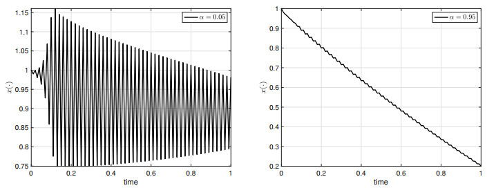
We consider the terminal state-constrained optimal control problem for Volterra integral equations with singular kernels. A singular kernel introduces abnormal behavior of the state trajectory with respect to the parameter of $ \alpha \in (0, 1) $. Our state equation covers various state dynamics such as any types of classical Volterra integral equations with nonsingular kernels, (Caputo) fractional differential equations, and ordinary differential state equations. We prove the maximum principle for the corresponding state-constrained optimal control problem. In the proof of the maximum principle, due to the presence of the (terminal) state constraint and the control space being only a separable metric space, we have to employ the Ekeland variational principle and the spike variation technique, together with the intrinsic properties of distance function and the generalized Gronwall's inequality, to obtain the desired necessary conditions for optimality. The maximum principle of this paper is new in the optimal control problem context and its proof requires a different technique, compared with that for classical Volterra integral equations studied in the existing literature.
Citation: Jun Moon. A Pontryagin maximum principle for terminal state-constrained optimal control problems of Volterra integral equations with singular kernels[J]. AIMS Mathematics, 2023, 8(10): 22924-22943. doi: 10.3934/math.20231166
We consider the terminal state-constrained optimal control problem for Volterra integral equations with singular kernels. A singular kernel introduces abnormal behavior of the state trajectory with respect to the parameter of $ \alpha \in (0, 1) $. Our state equation covers various state dynamics such as any types of classical Volterra integral equations with nonsingular kernels, (Caputo) fractional differential equations, and ordinary differential state equations. We prove the maximum principle for the corresponding state-constrained optimal control problem. In the proof of the maximum principle, due to the presence of the (terminal) state constraint and the control space being only a separable metric space, we have to employ the Ekeland variational principle and the spike variation technique, together with the intrinsic properties of distance function and the generalized Gronwall's inequality, to obtain the desired necessary conditions for optimality. The maximum principle of this paper is new in the optimal control problem context and its proof requires a different technique, compared with that for classical Volterra integral equations studied in the existing literature.

| [1] |
O. P. Agrawal, A general formulation and solution scheme for fractional optimal control problems, Nonlinear Dyn., 38 (2004), 323–337. https://doi.org/10.1007/s11071-004-3764-6 doi: 10.1007/s11071-004-3764-6

|
| [2] |
G. V. Alekseev, R. V. Brizitskii, Analysis of the boundary value and control problems for nonlinear reaction-diffusion-convection equation, J. Sib. Fed. Univ. Math. Phys., 14 (2021), 452–462. https://doi.org/10.17516/1997-1397-2021-14-4-452-462 doi: 10.17516/1997-1397-2021-14-4-452-462
|
| [3] |
T. S. Angell, On the optimal control of systems governed by nonlinear Volterra equations, J. Optim. Theory Appl., 19 (1976), 29–45. https://doi.org/10.1007/BF00934050 doi: 10.1007/BF00934050
|
| [4] |
A. Arutyunov, D. Karamzin, A survey on regularity conditions for state-constrained optimal control problems and the non-degenerate maximum principle, J. Optim. Theory Appl., 184 (2020), 697–723. https://doi.org/10.1007/s10957-019-01623-7 doi: 10.1007/s10957-019-01623-7
|
| [5] |
E. S. Baranovskii, Optimal boundary control of nonlinear-viscous fluid flows, Sb. Math., 211 (2020), 505–520. https://doi.org/10.1070/SM9246 doi: 10.1070/SM9246
|
| [6] |
E. S. Baranovskii, The optimal start control problem for $\text2D$ Boussinesq equations, Izv. Math., 86 (2022), 221–242. https://doi.org/10.1070/IM9099 doi: 10.1070/IM9099
|
| [7] |
S. A. Belbas, A new method for optimal control of Volterra integral equations, Appl. Math. Comput., 189 (2007), 1902–1915. https://doi.org/10.1016/j.amc.2006.12.077 doi: 10.1016/j.amc.2006.12.077
|
| [8] |
M. Bergounioux, L. Bourdin, Pontryagin maximum principle for general Caputo fractional optimal control problems with Bolza cost and terminal constraints, ESAIM: COCV, 26 (2020), 35. https://doi.org/10.1051/cocv/2019021 doi: 10.1051/cocv/2019021
|
| [9] |
P. Bettiol, L. Bourdin, Pontryagin maximum principle for state constrained optimal sampled-data control problems on time scales, ESAIM: COCV, 27 (2020), 51. https://doi.org/10.1051/cocv/2021046 doi: 10.1051/cocv/2021046
|
| [10] | V. I. Bogachev, Measure theory, Springer, 2000. |
| [11] |
J. F. Bonnans, The shooting approach to optimal control problems, IFAC Proc. Vol., 46 (2013), 281–292. https://doi.org/10.3182/20130703-3-FR-4038.00158 doi: 10.3182/20130703-3-FR-4038.00158
|
| [12] |
J. F. Bonnans, C. de la Vega, Optimal control of state constrained integral equations, Set-Valued Anal., 18 (2010), 307–326. https://doi.org/10.1007/s11228-010-0154-8 doi: 10.1007/s11228-010-0154-8
|
| [13] |
J. F. Bonnans, C. de la Vega, X. Dupuis, First- and second-order optimality conditions for optimal control problems of state constrained integral equations, J. Optim. Theory Appl., 159 (2013), 1–40. https://doi.org/10.1007/s10957-013-0299-3 doi: 10.1007/s10957-013-0299-3
|
| [14] | L. Bourdin, A class of fractional optimal control problems and fractional Pontryagin's systems. Existence of a fractional Noether's theorem, arXiv, 2012. https://doi.org/10.48550/arXiv.1203.1422 |
| [15] | L. Bourdin, Note on Pontryagin maximum principle with running state constraints and smooth dynamics–Proof based on the Ekeland variational principle, arXiv, 2016. https://doi.org/10.48550/arXiv.1604.04051 |
| [16] |
L. Bourdin, G. Dhar, Optimal sampled-data controls with running inequality state constraints: Pontryagin maximum principle and bouncing trajectory phenomenon, Math. Program., 191 (2022), 907–951. https://doi.org/10.1007/s10107-020-01574-2 doi: 10.1007/s10107-020-01574-2
|
| [17] | B. Brunner, Volterra integral equations: an introduction to theory and applications, Cambridge University Press, 2017. https://doi.org/10.1017/9781316162491 |
| [18] |
C. Burnap, M. A. Kazemi, Optimal control of a system governed by nonlinear Volterra integral equations with delay, IMA J. Math. Control Inf., 16 (1999), 73–89. https://doi.org/10.1093/imamci/16.1.73 doi: 10.1093/imamci/16.1.73
|
| [19] | T. A. Burton, Volterra integral and differential equations, 2 Eds., Elsevier Science Inc., 2005. |
| [20] |
D. A. Carlson, An elementary proof of the maximum principle for optimal control problems governed by a Volterra integral equation, J. Optim. Theory Appl., 54 (1987), 43–61. https://doi.org/10.1007/BF00940404 doi: 10.1007/BF00940404
|
| [21] | F. H. Clarke, Optimization and nonsmooth analysis, SIAM, 1990. |
| [22] |
A. V. Dmitruk, N. P. Osmolovskii, Necessary conditions for a weak minimum in optimal control problems with integral equations subject to state and mixed constraints, SIAM J. Control Optim., 52 (2014), 3437–3462. https://doi.org/10.1137/130921465 doi: 10.1137/130921465
|
| [23] |
A. V. Dmitruk, N. P. Osmolovskii, Necessary conditions for a weak minimum in a general optimal control problem with integral equations on a variable time interval, Math. Control Relat. F., 7 (2017), 507–535. https://doi.org/10.3934/mcrf.2017019 doi: 10.3934/mcrf.2017019
|
| [24] | T. M. Flett, Differential analysis, Cambridge University Press, 1980. https://doi.org/10.1017/CBO9780511897191 |
| [25] |
M. I. Gomoyunov, Dynamic programming principle and Hamilton-Jacobi-Bellman equations for fractional-order systems, SIAM J. Control Optim., 58 (2020), 3185–3211. https://doi.org/10.1137/19M1279368 doi: 10.1137/19M1279368
|
| [26] |
Y. Hamaguchi, Infinite horizon backward stochastic Volterra integral equations and discounted control problems, ESAIM: COCV, 101 (2021), 1–47. https://doi.org/10.1051/cocv/2021098 doi: 10.1051/cocv/2021098
|
| [27] |
Y. Hamaguchi, On the maximum principle for optimal control problems of stochastic Volterra integral equations with delay, Appl. Math. Optim., 87 (2023), 42. https://doi.org/10.1007/s00245-022-09958-w doi: 10.1007/s00245-022-09958-w
|
| [28] | S. Han, P. Lin, J. Yong, Causal state feedback representation for linear quadratic optimal control problems of singular Volterra integral equations, Math. Control Relat. F., 2022. https://doi.org/10.3934/mcrf.2022038 |
| [29] |
R. F. Hartl, S. P. Sethi, R. G. Vickson, A survey of the maximum principle for optimal control problems with state constraints, SIAM J. Control Optim., 37 (1995), 181–218. https://doi.org/10.1137/1037043 doi: 10.1137/1037043
|
| [30] |
M. I. Kamien, E. Muller, Optimal control with integral state equations, Rev. Econ. Stud., 43 (1976), 469–473. https://doi.org/10.2307/2297225 doi: 10.2307/2297225
|
| [31] |
R. Kamocki, On the existence of optimal solutions to fractional optimal control problems, Appl. Math. Comput., 235 (2014), 94–104. https://doi.org/10.1016/j.amc.2014.02.086 doi: 10.1016/j.amc.2014.02.086
|
| [32] | A. A. Kilbas, H. M. Srivastava, J. J. Trujillo, Theory and applications of fractional differential equations, Elsevier, 2006. |
| [33] | X. Li, J. Yong, Optimal control theory for infinite dimensional systems, 1 Ed., Boston: Birkhäuser Boston, 1995. https://doi.org/10.1007/978-1-4612-4260-4 |
| [34] |
P. Lin, J. Yong, Controlled singular Volterra integral equations and Pontryagin maximum principle, SIAM J. Control Optim., 58 (2020), 136–164. https://doi.org/10.1137/19M124602X doi: 10.1137/19M124602X
|
| [35] |
N. G. Medhin, Optimal processes governed by integral equation equations with unilateral constraints, J. Math. Anal. Appl., 129 (1988), 269–283. https://doi.org/10.1016/0022-247X(88)90248-X doi: 10.1016/0022-247X(88)90248-X
|
| [36] |
H. K. Moffatt, Helicity and singular structures in fluid dynamics, Proc. Natl. Acad. Sci., 111 (2014), 3663–3670. https://doi.org/10.1073/pnas.1400277111 doi: 10.1073/pnas.1400277111
|
| [37] |
J. Moon, The risk-sensitive maximum principle for controlled forward-backward stochastic differential equations, Automatica, 120 (2020), 109069. https://doi.org/10.1016/j.automatica.2020.109069 doi: 10.1016/j.automatica.2020.109069
|
| [38] | A. Ruszczynski, Nonlinear optimization, Princeton University Press, 2006. |
| [39] |
C. de la Vega, Necessary conditions for optimal terminal time control problems governed by a Volterra integral equation, J. Optim. Theory Appl., 130 (2006), 79–93. https://doi.org/10.1007/s10957-006-9087-7 doi: 10.1007/s10957-006-9087-7
|
| [40] |
V. R. Vinokurov, Optimal control of processes described by integral equations III, SIAM J. Control, 7 (1969), 324–355. https://doi.org/10.1137/0307024 doi: 10.1137/0307024
|
| [41] | R. Vinter, Optimal control, Birkhäuser, 2000. |
| [42] |
T. Wang, Linear quadratic control problems of stochastic integral equations, ESAIM: COCV, 24 (2018), 1849–1879. https://doi.org/10.1051/cocv/2017002 doi: 10.1051/cocv/2017002
|
| [43] | J. Yong, X. Y. Zhou, Stochastic controls: Hamiltonian systems and HJB equations, New York: Springer Science$+$Business Media, 1999. https://doi.org/10.1007/978-1-4612-1466-3 |
Figures(5)

Jun Moon. A Pontryagin maximum principle for terminal state-constrained optimal control problems of Volterra integral equations with singular kernels[J]. AIMS Mathematics, 2023, 8(10): 22924-22943. doi: 10.3934/math.20231166


 DownLoad: