Pathfinding algorithm based on rotated block AOR technique in structured environment

A'qilah Ahmad Dahalan; Azali Saudi; A'qilah Ahmad Dahalan; Azali Saudi

doi:10.3934/math.2022643

AIMS Mathematics

2022, Volume 7, Issue 7: 11529-11550. doi: 10.3934/math.2022643

Previous Article Next Article

Research article

Pathfinding algorithm based on rotated block AOR technique in structured environment

A'qilah Ahmad Dahalan ^{1,2
,
,},
Azali Saudi ³

1.
Department of Mathematics, Universiti Pertahanan Nasional Malaysia, Kuala Lumpur, Malaysia
2.
CONFIRM Centre for SMART Manufacturing, University of Limerick, Limerick, Ireland
3.
Faculty of Computing and Informatics, Universiti Malaysia Sabah, Kota Kinabalu, Malaysia

Received: 24 November 2021 Revised: 07 March 2022 Accepted: 24 March 2022 Published: 14 April 2022
MSC : 35J05, 65D19, 65K05, 65M06

Harmonic potential fields are commonly used as guidance in a global approach for self-directed robot pathfinding. These harmonic potentials are generated using Laplace's equation solutions. The computation of these harmonic potentials often requires the use of immense amounts of computing resources. This study introduces a numerical technique called Rotated Block Accelerated Over-Relaxation (AOR), also known as Explicit Decoupled Group AOR (EDGAOR), to deal with pathfinding problem. Several robot navigation simulations were performed in a static, structured, known indoor environment to validate the efficiency of the suggested approach. The paths generated by the simulations are shown using several different starting and target positions. The performance of the proposed approach in computing harmonic potentials for solving pathfinding problems is also discussed.
- algorithms,
- Laplace's equation,
- half-sweep iterative method,
- numerical analysis,
- collision free,
- optimal path
Citation: A'qilah Ahmad Dahalan, Azali Saudi. Pathfinding algorithm based on rotated block AOR technique in structured environment[J]. AIMS Mathematics, 2022, 7(7): 11529-11550. doi: 10.3934/math.2022643

Related Papers:

Abstract

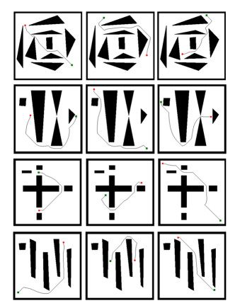
Harmonic potential fields are commonly used as guidance in a global approach for self-directed robot pathfinding. These harmonic potentials are generated using Laplace's equation solutions. The computation of these harmonic potentials often requires the use of immense amounts of computing resources. This study introduces a numerical technique called Rotated Block Accelerated Over-Relaxation (AOR), also known as Explicit Decoupled Group AOR (EDGAOR), to deal with pathfinding problem. Several robot navigation simulations were performed in a static, structured, known indoor environment to validate the efficiency of the suggested approach. The paths generated by the simulations are shown using several different starting and target positions. The performance of the proposed approach in computing harmonic potentials for solving pathfinding problems is also discussed.

References

[1]	B. Patle, G. Babu L, A. Pandey, D. Parhi, A. Jagadeesh, A review: on path planning strategies for navigation of mobile robot, Def. Technol., 15 (2019), 582-606. http://dx.doi.org/10.1016/j.dt.2019.04.011 doi: 10.1016/j.dt.2019.04.011
[2]	N. Buniyamin, N. Sariff, W. Wan Ngah, Z. Mohamad, Robot global path planning overview and a variation of ant colony system algorithm, International Journal of Mathematics and Computers in Simulation, 5 (2011), 9-16.
[3]	S. Sasaki, A practical computational technique for mobile robot navigation, Proceedings of the IEEE International Conference on Control Applications, 1998, 1323-1327. http://dx.doi.org/10.1109/CCA.1998.721675 doi: 10.1109/CCA.1998.721675
[4]	C. Connolly, R. Gruppen, The applications of harmonic functions to robotics, J. Robotic Syst., 10 (1993), 931-946. http://dx.doi.org/10.1002/rob.4620100704 doi: 10.1002/rob.4620100704
[5]	O. Khatib, Real-time obstacle avoidance for manipulators and mobile robots, Proceedings of IEEE International Conference on Robotics and Automation, 1985,500-505. http://dx.doi.org/10.1109/ROBOT.1985.1087247 doi: 10.1109/ROBOT.1985.1087247
[6]	S. Waydo, R. Murray, Vehicle motion planning using stream functions, Proceedings of IEEE International Conference on Robotics and Automation, 2003, 2484-2491. http://dx.doi.org/10.1109/ROBOT.2003.1241966 doi: 10.1109/ROBOT.2003.1241966
[7]	H. Ghassemi, S. Panahi, A. Kohansal, Solving the Laplace's equation by the FDM and BEM using mixed boundary conditions, American Journal of Applied Mathematics and Statistics, 4 (2016), 37-42. http://dx.doi.org/10.12691/ajams-4-2-2 doi: 10.12691/ajams-4-2-2
[8]	P. Kuo, C. Wang, H. Chou, J. Liu, A real-time streamline-based obstacle avoidance system for curvature-constrained nonholonomic mobile robots, Proceedings of 6th International Symposium on Advanced Control of Industrial Processes, 2017,618-623. http://dx.doi.org/10.1109/ADCONIP.2017.7983851 doi: 10.1109/ADCONIP.2017.7983851
[9]	C. Connolly, J. Burns, R. Weiss, Path planning using Laplace's equation, Proceedings of IEEE International Conference on Robotics and Automation, 1990, 2102-2106. http://dx.doi.org/10.1109/ROBOT.1990.126315 doi: 10.1109/ROBOT.1990.126315
[10]	J. Barraquand, B. Langlois, J. Latombe, Numerical potential field techniques for robot path planning, IEEE T. Syst. Man Cyb., 22 (1992), 224-241. http://dx.doi.org/10.1109/21.148426 doi: 10.1109/21.148426
[11]	M. Karnik, B. Dasgupta, V. Eswaran, A comparative study of Dirichlet and Neumann conditions for path planning through harmonic functions, In: Lecture notes in computer science, Berlin: Springer, 2002,442-451. http://dx.doi.org/10.1007/3-540-46080-2_46
[12]	N. Montes, F. Chinesta, M. Mora, A. Falco, L. Hilario, N. Rosillo, E. Nadal, Real-time path planning based on harmonic functions under a proper generalized decomposition-based framework, Sensors, 21 (2021), 3943. http://dx.doi.org/10.3390/s21123943 doi: 10.3390/s21123943
[13]	A. Falco, L. Hilario, N. Montes, M. Mora, E. Nadal, A path planning algorithm for a dynamic environment based on proper generalized decomposition, Mathematics, 8 (2020), 2245. http://dx.doi.org/10.3390/math8122245 doi: 10.3390/math8122245
[14]	K. Al-Khaled, Numerical solutions of the Laplace's equation, Appl. Math. Comput., 170 (2005), 1271-1283. http://dx.doi.org/10.1016/j.amc.2005.01.018
[15]	K. Shivaram, H. Jyothi, Finite element approach for numerical integration over family of eight node linear quadrilateral element for solving Laplace equation, Materials Today: Proceedings, 46 (2021), 4336-4340. http://dx.doi.org/10.1016/j.matpr.2021.03.437 doi: 10.1016/j.matpr.2021.03.437
[16]	Y. Liu, C. Fan, W. Yeih, C. Ku, C. Chu, Numerical solutions of two-dimensional Laplace and biharmonic equations by the localized Trefftz method, Comput. Math. Appl., 88 (2021), 120-134. http://dx.doi.org/10.1016/j.camwa.2020.09.023 doi: 10.1016/j.camwa.2020.09.023
[17]	A. Abdullah, The four point explicit decoupled group (EDG) method: a fast poison solver, Int. J. Comput. Math., 38 (1991), 61-70. http://dx.doi.org/10.1080/00207169108803958 doi: 10.1080/00207169108803958
[18]	A. Saudi, J. Sulaiman, Half-sweep Gauss-Seidel (HSGS) iterative method for robot path planning, Proceedings of the 3rd International Conference on Informatics and Technology, 2009, 34-39.
[19]	M. Muthuvalu, J. Sulaiman, Half-sweep arithmetic mean method with composite trapezoidal scheme for solving linear Fredholm integral equations, Appl. Math. Comput., 217 (2011), 5442-5448. http://dx.doi.org/10.1016/j.amc.2010.12.013 doi: 10.1016/j.amc.2010.12.013
[20]	M. Muthuvalu, T. Htun, E. Aruchunan, M. Ali, J. Sulaiman, Performance analysis of half-sweep successive over-relaxation iterative method for solving four-point composite closed newton-cotes system, Proceedings of 7th International Conference on Intelligent Systems, Modelling and Simulation, 2016,375-379. http://dx.doi.org/10.1109/ISMS.2016.84 doi: 10.1109/ISMS.2016.84
[21]	S. Matsui, H. Nagahara, R. Taniguchi, Half-sweep imaging for depth from defocus, Image Vision Comput., 32 (2014), 954-964. http://dx.doi.org/10.1016/j.imavis.2014.09.001 doi: 10.1016/j.imavis.2014.09.001
[22]	F. Muhiddin, J. Sulaiman, A. Sunarto, Solving time-fractional parabolic equations with the four point-HSEGKSOR iteration, In: Lecture notes in electrical engineering, Singapore: Springer, 2021,281-293. http://dx.doi.org/10.1007/978-981-33-4069-5_24
[23]	A. Dahalan, A. Saudi, Rotated TOR-5P Laplacian iteration path navigation for obstacle avoidance in stationary indoor simulation, In: Advances in intelligent systems and computing, Cham: Springer, 2021,285-295. http://dx.doi.org/10.1007/978-3-030-70917-4_27
[24]	J. Sulaiman, M. Hassan, M. Othman, The half-sweep iterative alternating decomposition explicit (HSIADE) method for diffusion equation, In: Lecture notes in computer sciences, Berlin: Springer, 2004, 57-63. http://dx.doi.org/10.1007/978-3-540-30497-5_10
[25]	J. Sulaiman, M. Othman, M. Hassan, Nine point-EDGSOR iterative method for the finite element solution of 2D Poisson equations, In: Lecture notes in computer sciences, Berlin: Springer, 2009,764-774. http://dx.doi.org/10.1007/978-3-642-02454-2_59
[26]	A. Saudi, J. Sulaiman, Robot path planning using Laplacian behaviour-based control (LBBC) via half-sweep SOR, Proceedings of the International Conference on Technological Advances in Electrical, Electronics and Computer Engineering, 2013,424-429. http://dx.doi.org/10.1109/TAEECE.2013.6557312 doi: 10.1109/TAEECE.2013.6557312
[27]	A. Ibrahim, A. Abdullah, Solving the two dimensional diffusion equation by the four point explicit decoupled group (EDG) iterative method, Int. J. Comput. Math., 58 (1995), 253-263. http://dx.doi.org/10.1080/00207169508804447 doi: 10.1080/00207169508804447
[28]	D. Evans, Group explicit iterative methods for solving large linear systems, Int. J. Comput. Math., 17 (1985), 81-108. http://dx.doi.org/10.1080/00207168508803452 doi: 10.1080/00207168508803452
[29]	G. Dahlquist, A. Bjorck, Numerical methods, New Jersey: Prentice Hall, 1974.
[30]	W. Yousif, D. Evans, Explicit group over-relaxation methods for solving elliptic partial differential equations, Math. Comput. Simulat., 28 (1986), 453-466. http://dx.doi.org/10.1016/0378-4754(86)90040-6 doi: 10.1016/0378-4754(86)90040-6
[31]	D. Young, Iterative methods for solving partial difference equations of elliptic type, PhD Thesis, Harvard University, 1950.
[32]	D. Young, Iterative methods for solving partial difference equations of elliptic type, Trans. Amer. Math. Soc., 76 (1954), 92-111. http://dx.doi.org/10.2307/1990745 doi: 10.2307/1990745
[33]	D. Young, Iterative solution of large linear systems, London: Academic Press, 1971.
[34]	A. Hadjidimos, Accelerated overrelaxation method, Math. Comput., 32 (1978), 149-157. http://dx.doi.org/10.2307/20006264 doi: 10.2307/20006264
[35]	M. Martins, W. Yousif, D. Evans, Explicit group AOR method for solving elliptic partial differential equations, Neural, Parallel & Scientific Computations, 10 (2002), 411-422.
[36]	M. Othman, A. Abdullah, An efficient four points modified explicit group poisson solver, Int. J. Comput. Math., 76 (2000), 203-217. http://dx.doi.org/10.1080/00207160008805020 doi: 10.1080/00207160008805020
[37]	N. Ali, S. Lee, Group accelerated OverRelaxation methods on rotated grid, Appl. Math. Comput., 191 (2007), 533-542. http://dx.doi.org/10.1016/j.amc.2007.02.131 doi: 10.1016/j.amc.2007.02.131
[38]	K. Wray, D. Ruiken, R. Grupen, S. Zilberstein, Log-space harmonic function path planning, Proceedings of IEEE/RSJ International Conference on Intelligent Robots and Systems, 2016, 1511-1516. http://dx.doi.org/10.1109/IROS.2016.7759245 doi: 10.1109/IROS.2016.7759245
[39]	J. Navnit, The application of sixth order accurate parallel quarter sweep alternating group explicit algorithm for nonlinear boundary value problems with singularity, Proceedings of International Conference on Methods and Models in Computer Science, 2010, 76-80. http://dx.doi.org/10.1109/ICM2CS.2010.5706722 doi: 10.1109/ICM2CS.2010.5706722
[40]	A. Sunarto, J. Sulaiman, Investigation of fractional diffusion equation via QSGS iterations, J. Phys. Conf. Ser., 1179 (2019), 012014. http://dx.doi.org/10.1088/1742-6596/1179/1/012014 doi: 10.1088/1742-6596/1179/1/012014
[41]	J. Lung, J. Sulaiman, On quarter-sweep finite difference scheme for one-dimensional porous medium equations, International Journal of Applied Mathematics, 33 (2020), 439-450. http://dx.doi.org/10.12732/ijam.v33i3.6 doi: 10.12732/ijam.v33i3.6

Reader Comments

Your name:*

Email:*
© 2022 the Author(s), licensee AIMS Press. This is an open access article distributed under the terms of the Creative Commons Attribution License (http://creativecommons.org/licenses/by/4.0)