Dynamics and optimal control of an online game addiction model with considering family education

Youming Guo; Tingting Li; Youming Guo; Tingting Li

doi:10.3934/math.2022208

AIMS Mathematics

2022, Volume 7, Issue 3: 3745-3770. doi: 10.3934/math.2022208

Previous Article Next Article

Research article

Dynamics and optimal control of an online game addiction model with considering family education

Youming Guo ^1,2,
Tingting Li ^{1,2
,
,}

1.
College of Science, Guilin University of Technology, Guilin, Guangxi 541004, China
2.
Guangxi Colleges and Universities Key Laboratory of Applied Statistics, Guilin University of Technology, Guilin, Guangxi 541004, China

Received: 15 August 2021 Accepted: 06 December 2021 Published: 08 December 2021
MSC : 34D23, 49J15

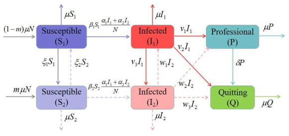
The problem of online game addiction among teenagers is becoming more and more serious in many parts of the world. Many of them are addicted to online games due to the lack of family education, which is an important factor that can not be ignored. To explore the optimal strategy for controlling the spread of game addiction, a new dynamic model of teenagers' online game addiction with considering family education is developed. Firstly, we perform a qualitative dynamic analysis of the model. We study the nonnegativity and boundedness of solutions, the basic reproduction number $ R_{0} $, and the existence and stability of equilibria. We then consider a model with control measures of family education, isolation and treatment, and obtain the expression of optimal control. In the numerical simulation, we study the global sensitivity analysis by the combination of Latin Hypercube Sampling (LHS) and partial rank correlation coefficient (PRCC) techniques, and show the relationship between $ R_{0} $ and each parameter. Then the forward backward sweep method with fourth order Runge-Kutta is used to simulate the control strategy in each scenario. Finally, the optimal control strategy is obtained by comparing incremental cost-effectiveness ratio (ICER) and infection averted ratio (IAR) under all strategies. The results show that with sufficient financial resources, adding the family education measures can help more teenagers avoid being addicted to games and control the spread of game addiction more effectively.
- online game addiction model,
- family education,
- dynamics,
- forward-backward sweep method,
- optimal control,
- cost-effectiveness analysis
Citation: Youming Guo, Tingting Li. Dynamics and optimal control of an online game addiction model with considering family education[J]. AIMS Mathematics, 2022, 7(3): 3745-3770. doi: 10.3934/math.2022208

Related Papers:

Abstract

The problem of online game addiction among teenagers is becoming more and more serious in many parts of the world. Many of them are addicted to online games due to the lack of family education, which is an important factor that can not be ignored. To explore the optimal strategy for controlling the spread of game addiction, a new dynamic model of teenagers' online game addiction with considering family education is developed. Firstly, we perform a qualitative dynamic analysis of the model. We study the nonnegativity and boundedness of solutions, the basic reproduction number $ R_{0} $, and the existence and stability of equilibria. We then consider a model with control measures of family education, isolation and treatment, and obtain the expression of optimal control. In the numerical simulation, we study the global sensitivity analysis by the combination of Latin Hypercube Sampling (LHS) and partial rank correlation coefficient (PRCC) techniques, and show the relationship between $ R_{0} $ and each parameter. Then the forward backward sweep method with fourth order Runge-Kutta is used to simulate the control strategy in each scenario. Finally, the optimal control strategy is obtained by comparing incremental cost-effectiveness ratio (ICER) and infection averted ratio (IAR) under all strategies. The results show that with sufficient financial resources, adding the family education measures can help more teenagers avoid being addicted to games and control the spread of game addiction more effectively.

References

[1]	The 46rd statistical report on internet development in China, Cyberspace Administration of China, 2020. Available from: http://www.cac.gov.cn/2020-09/29/c_1602939918747816.htm.
[2]	D. Loton, E. Borkoles, D. Lubman, R. Polman, Video game addiction, engagement and symptoms of stress, depression and anxiety: The mediating role of coping, Int. J. Ment. Health. Ad., 14 (2016), 565–578. doi: 10.1007/s11469-015-9578-6. doi: 10.1007/s11469-015-9578-6
[3]	Z. Lu, From e-heroin to e-sports: The development of competitive gaming in China, Int. J. Hist. Sport, 33 (2016), 2186–2206. doi: 10.1080/09523367.2017.1358167. doi: 10.1080/09523367.2017.1358167
[4]	X. Yang, X. Jiang, P. Mo, Y. Cai, L. Ma, J. Lau, Prevalence and interpersonal correlates of internet gaming disorders among Chinese adolescents, Int. J. Environ. Res. Public Health, 17 (2020), 579. doi: 10.3390/ijerph17020579. doi: 10.3390/ijerph17020579
[5]	B. Egliston, Watch to win? E-sport, broadcast expertise and technicity in Dota 2, Convergence, 26 (2020), 1174–1193. doi: 10.1177/1354856519851180. doi: 10.1177/1354856519851180
[6]	R. Liu, J. Wu, H. Zhu, Media/psychological impact on multiple outbreaks of emerging infectious diseases, Comput. Math. Method. M., 8 (2007), 153–164. doi: 10.1080/17486700701425870. doi: 10.1080/17486700701425870
[7]	A. Atangana, M. A. Khan, Fatmawati, Modeling and analysis of competition model of bank data with fractal-fractional Caputo-Fabrizio operator, Alex. Eng. J., 59 (2020), 1985–1998. doi: 10.1016/j.aej.2019.12.032. doi: 10.1016/j.aej.2019.12.032
[8]	D. Baleanu, A. Jajarmi, H. Mohammadi, S. Rezapour, A new study on the mathematical modelling of human liver with Caputo–Fabrizio fractional derivative, Chaos Soliton. Fract., 134 (2020), 109705. doi: 10.1016/j.chaos.2020.109705. doi: 10.1016/j.chaos.2020.109705
[9]	Y. Li, L. Wang, L. Pang, S. Liu, The data fitting and optimal control of a hand, foot and mouth disease (HFMD) model with stage structure, Appl. Math. Comput., 276 (2016), 61–74. doi: 10.1016/j.amc.2015.11.090. doi: 10.1016/j.amc.2015.11.090
[10]	O. Sharomi, A. B. Gumel, Curtailing smoking dynamics: A mathematical modeling approach, Appl. Math. Comput., 195 (2008), 475–499. doi: 10.1016/j.amc.2007.05.012. doi: 10.1016/j.amc.2007.05.012
[11]	H. Huo, F. Cui, H. Xiang, Dynamics of an SAITS alcoholism model on unweighted andweighted networks, Physica A, 496 (2018), 249–262. doi: 10.1016/j.physa.2018.01.003. doi: 10.1016/j.physa.2018.01.003
[12]	J. Zhao, L. Yang, X. Zhong, X. Yang, Y. Wu, Y. Tang, Minimizing the impact of a rumor via isolation and conversion, Physica A, 526 (2019), 120867. doi: 10.1016/j.physa.2019.04.103. doi: 10.1016/j.physa.2019.04.103
[13]	T. Li, Y. Guo, Optimal control of an online game addiction model with positive and negative media reports, J. Appl. Math. Comput., 66 (2021), 599–619. doi: 10.1007/s12190-020-01451-3. doi: 10.1007/s12190-020-01451-3
[14]	R. Viriyapong, M. Sookpiam, Education campaign and family understanding affect stability and qualitative behavior of an online game addiction model for children and youth in Thailand, Math. Method. Appl. Sci., 42 (2019), 6906–6916. doi: 10.1002/mma.5796. doi: 10.1002/mma.5796
[15]	Y. Tian, X. Ding, Rumor spreading model with considering debunking behavior in emergencies, Appl. Math. Comput., 363 (2019), 124599. doi: 10.1016/j.amc.2019.124599. doi: 10.1016/j.amc.2019.124599
[16]	H. Huo, H. Xue, H. Xiang, Dynamics of an alcoholism model on complex networks with community structure and voluntary drinking, Physica A, 505 (2018), 880–890. doi: 10.1016/j.physa.2018.04.024. doi: 10.1016/j.physa.2018.04.024
[17]	W. Liu, S Zhong, Web malware spread modelling and optimal control strategies, Sci. Rep-UK, 7 (2017), 42308. doi: 10.1038/srep42308. doi: 10.1038/srep42308
[18]	Y. Guo, T. Li, Optimal control and stability analysis of an online game addiction model with two stages, Math. Method. Appl. Sci., 43 (2020), 4391–4408. doi: 10.1002/mma.6200. doi: 10.1002/mma.6200
[19]	H. Seno, A mathematical model of population dynamics for the internet gaming addiction, Nonlinear Anal-Model., 26 (2021), 861–883. doi: 10.15388/namc.2021.26.24177. doi: 10.15388/namc.2021.26.24177
[20]	D. Kada, B. Khajji, O. Balatif, M. Rachik, E. H. Labriji, Optimal control approach of discrete mathematical modeling of the spread of gaming disorder in morocco and cost-effectiveness analysis, Discrete Dyn. Nat. Soc., 2021 (2021), 5584315. doi: 10.1155/2021/5584315. doi: 10.1155/2021/5584315
[21]	Y. Guo, T. Li, Optimal control strategies for an online game addiction model with low and high risk exposure, Discrete Cont. Dyn. B, 26 (2021), 5355–5382. doi: 10.3934/dcdsb.2020347. doi: 10.3934/dcdsb.2020347
[22]	M. C. Zara, L. H. A. Monteiro, The negative impact of technological advancements on mental health: An epidemiological approach, Appl. Math. Comput., 396 (2021), 125905. doi: 10.1016/j.amc.2020.125905. doi: 10.1016/j.amc.2020.125905
[23]	M. A. Khan, S. W. Shah, S. Ullah, J. F. Gómez-Aguilar, A dynamical model of asymptomatic carrier Zika virus with optimal control strategies, Nonlinear Anal. Real., 50 (2019), 144–170. doi: 10.1016/j.nonrwa.2019.04.006. doi: 10.1016/j.nonrwa.2019.04.006
[24]	M. A. Khan, S. A. A. Shah, S. Ullah, K. O. Okosun, M. Farooq, Optimal control analysis of the effect of treatment, isolation and vaccination on hepatitis B virus, J. Biol. Syst., 28 (2020), 351–376. doi: 10.1142/S0218339020400057. doi: 10.1142/S0218339020400057
[25]	S. Ullah, O. Ullah, M. A. Khan, T. Gul, Optimal control analysis of tuberculosis (TB) with vaccination and treatment, Eur. Phys. J. Plus, 135 (2020), 602. doi: 10.1140/epjp/s13360-020-00615-1. doi: 10.1140/epjp/s13360-020-00615-1
[26]	L. Pang, S. Liu, X. Zhang, T. Tian, The cost-effectiveness analysis and optimal strategy of the tobacco control, Comput. Math. Method. M., 2019 (2019), 8189270. doi: 10.1155/2019/8189270. doi: 10.1155/2019/8189270
[27]	S. Zhang, X. Xu, Dynamic analysis and optimal control for a model of hepatitis C with treatment, Commun. Nonlinear Sci., 46 (2017), 14–25. doi: 10.1016/j.cnsns.2016.10.017. doi: 10.1016/j.cnsns.2016.10.017
[28]	P. M. Mwamtobe, S. M. Simelane, S. Abelman, J. M. Tchuench, Optimal control of intervention strategies in malaria-tuberculosis co-infection with relapse, Int. J. Biomath., 11 (2018), 1850017. doi: 10.1142/S1793524518500171. doi: 10.1142/S1793524518500171
[29]	D. N. Greenfield, Treatment considerations in internet and video game addiction, Child Adol. Psych. Cl., 27 (2018), 327–344. doi: 10.1016/j.chc.2017.11.007. doi: 10.1016/j.chc.2017.11.007
[30]	K. H. Chen, J. L. Oliffe, M. T. Kelly, Internet gaming disorder: An emergent health issue for men, Am. J. Men's Health, 12 (2018), 1151–1159. doi: 10.1177/1557988318766950. doi: 10.1177/1557988318766950
[31]	T. Li, Y. Guo, Stability and optimal control in a mathematical model of online game addiction, Filomat, 33 (2019), 5691–5711. doi: 10.2298/FIL1917691L. doi: 10.2298/FIL1917691L
[32]	H. Alrabaiah, M. A. Safi, M. H. DarAssi, B. Al-Hdaibat, S. Ullah, M. A. Khan, et al. {Optimal control analysis of hepatitis B virus with treatment and vaccination}, Results Phys., 19 (2020), 103599. doi: 10.1016/j.rinp.2020.103599. doi: 10.1016/j.rinp.2020.103599
[33]	S. Ullah, M. F. Khan, S. A. A. Shah, M. Farooq, M. A. Khan, M. B. Mamat, Optimal control analysis of vector-host model with saturated treatment, Eur. Phys. J. Plus, 135 (2020), 839. doi: 10.1140/epjp/s13360-020-00855-1. doi: 10.1140/epjp/s13360-020-00855-1
[34]	A. Boudaoui, Y. E. H. Moussa, Z. Hammouch, S. Ullah, A fractional-order model describing the dynamics of the novel coronavirus (COVID-19) with nonsingular kernel, Chaos Soliton. Fract., 146 (2021), 110859. doi: 10.1016/j.chaos.2021.110859. doi: 10.1016/j.chaos.2021.110859
[35]	S. Ullah, M. A. Khan, Modeling the impact of non-pharmaceutical interventions on the dynamics of novel coronavirus with optimal control analysis with a case study, Chaos Soliton. Fract., 139 (2020), 110075. doi: 10.1016/j.chaos.2020.110075. doi: 10.1016/j.chaos.2020.110075
[36]	S. Ullah, O. Ullah, M. A. Khan, T. Gul, Optimal control analysis of tuberculosis (TB) with vaccination and treatment, Eur. Phys. J. Plus, 135 (2020), 602. doi: 10.1140/epjp/s13360-020-00615-1. doi: 10.1140/epjp/s13360-020-00615-1
[37]	J. M. Heffernan, R. J. Smith, L. M. Wahl, Perspectives on the basic reproductive ratio, J. R. Soc. Interface, 2 (2005), 281–293. doi: 10.1098/rsif.2005.0042. doi: 10.1098/rsif.2005.0042
[38]	P. V. Driessche, J. Watmough, Reproduction numbers and sub-threshold endemic equilibria for compartmental models of disease transmission, Math. Biosci., 180 (2002), 29–48. doi: 10.1016/S0025-5564(02)00108-6. doi: 10.1016/S0025-5564(02)00108-6
[39]	J. P. La Salle, The stability of dynamical systems, Society for Industrial and Applied Mathematics, 1976.
[40]	L. Pontryagin, V. G. Boltyanskii, E. Mishchenko, The mathematical theory of optimal processes, 1961.
[41]	W. H. Fleming, R. W. Rishel, Deterministic and stochastic optimal control, New York: Springer-Verlag, 1975.
[42]	D. L. Lukes, Differential equations: Classical to controlled, New York: Academia Press, 1982.
[43]	M. McAsey, L. B. Mou, W. M. Han, Convergence of the forward-backward sweep method in optimal control, Comput. Optim. Appl., 53 (2012), 207–226. doi: 10.1007/s10589-011-9454-7. doi: 10.1007/s10589-011-9454-7
[44]	K. W. Blayneh, A. B. Gumel, S. Lenhart, T. Clayton, Backward bifurcation and optimal control in transmission dynamics of West Nile virus, B. Math. Biol., 72 (2010), 1006–1028. doi: 10.1007/s11538-009-9480-0. doi: 10.1007/s11538-009-9480-0
[45]	A. A. Momoh, A. Fügenschuh, Optimal control of intervention strategies and cost effectiveness analysis for a Zika virus model, Oper. Res. Health Care, 18 (2018), 99–111. doi: 10.1016/j.orhc.2017.08.004. doi: 10.1016/j.orhc.2017.08.004

Reader Comments

Your name:*

Email:*
© 2022 the Author(s), licensee AIMS Press. This is an open access article distributed under the terms of the Creative Commons Attribution License (http://creativecommons.org/licenses/by/4.0)