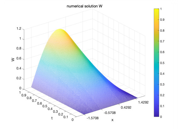
In this paper, an inverse problem of determining the space-dependent volatility from the observed market prices of options with different strikes is studied. Being different from other inverse volatility problem with classical parabolic equations, we apply the linearization method and introduce some variable substitutions to convert the original problem into an inverse source problem in a degenerate parabolic equation in a bounded area, from which an unknown volatility can be recovered and deficiencies caused by artificial truncation can be solved. Based on the optimal control framework, the problem is transformed into an optimization problem and the existence of the minimizer is established. After the necessary conditions are deduced, the uniqueness and stability of the minimizer are proved. Then, the Landweber iterative method is used to obtain a stable numerical solution of the inverse problem and some numerical experiments are also performed. The numerical results show that the algorithm which we proposed is robust and the unknown coefficient is recovered quite well.
Citation: Yilihamujiang Yimamu, Zui-Cha Deng, Liu Yang. An inverse volatility problem in a degenerate parabolic equation in a bounded domain[J]. AIMS Mathematics, 2022, 7(10): 19237-19266. doi: 10.3934/math.20221056
In this paper, an inverse problem of determining the space-dependent volatility from the observed market prices of options with different strikes is studied. Being different from other inverse volatility problem with classical parabolic equations, we apply the linearization method and introduce some variable substitutions to convert the original problem into an inverse source problem in a degenerate parabolic equation in a bounded area, from which an unknown volatility can be recovered and deficiencies caused by artificial truncation can be solved. Based on the optimal control framework, the problem is transformed into an optimization problem and the existence of the minimizer is established. After the necessary conditions are deduced, the uniqueness and stability of the minimizer are proved. Then, the Landweber iterative method is used to obtain a stable numerical solution of the inverse problem and some numerical experiments are also performed. The numerical results show that the algorithm which we proposed is robust and the unknown coefficient is recovered quite well.

| [1] | B. Dupire, Pricing with a smile, Risk, 7 (1994), 1–10. |
| [2] |
I. Bouchouev, V. Isakov, Uniqueness, stability and numerical methods for the inverse problem that arises in financial markets, Inverse Probl., 15 (1999), R95. http://doi.org/10.1088/0266-5611/15/3/201 doi: 10.1088/0266-5611/15/3/201

|
| [3] |
I. Bouchouev, V. Isakov, The inverse problem of option pricing, Inverse Probl., 13 (1997), L11. http://doi.org/10.1088/0266-5611/13/5/001 doi: 10.1088/0266-5611/13/5/001
|
| [4] |
L. S. Jiang, Y. S. Tao, Identifying the volatility of underlying assets from option prices, Inverse Probl., 17 (2001), 137. http://doi.org/10.1088/0266-5611/17/1/311 doi: 10.1088/0266-5611/17/1/311
|
| [5] |
L. Xiao, Z. L. Chen, Taxation problems in the dual model with capital injections, Acta. Math. Sci., 36 (2016), 187–192. http://doi.org/10.3969/j.issn.1003-3998.2016.01.016 doi: 10.3969/j.issn.1003-3998.2016.01.016
|
| [6] |
L. S. Jiang, Q. H. Chen, L. J. Wang, J. E. Zhang, A new well-posed algorism to recover implied local volatility, Quant. Financ., 3 (2003), 451–457. http://doi.org/10.1088/1469-7688/3/6/304 doi: 10.1088/1469-7688/3/6/304
|
| [7] |
L. S. Jiang, B. J. Bian, Identifying the principal coefficient of parabolic equations with non-divergent form, J. Phys.: Conf. Ser., 12 (2005), 58–65. http://doi.org/10.1088/1742-6596/12/1/006 doi: 10.1088/1742-6596/12/1/006
|
| [8] |
H. Egger, H. W. Engl, Tikhonov regularization applied to the inverse problem of option pricing: Convergence analysis and rates, Inverse Probl., 21 (2005), 1027. http://doi.org/10.1088/0266-5611/21/3/014 doi: 10.1088/0266-5611/21/3/014
|
| [9] |
Z. C. Deng, L. Yang, An inverse volatility problem of financial products linked with gold price, Bull. Iran. Math. Soc., 45 (2019), 1243–1267. http://doi.org/10.1007/s41980-018-00196-x doi: 10.1007/s41980-018-00196-x
|
| [10] |
V. Isakov, Recovery of time dependent volatility coefficient by linearization, Evol. Equ. Control. The., 3 (2017), 119–134. http://doi.org/10.1002/cpa.3160440203 doi: 10.1002/cpa.3160440203
|
| [11] |
Y. Ota, S. Kaji, Reconstruction of local volatility for the binary option model, J. Inverse Ill-Pose. P., 24 (2016), 727–741. http://doi.org/10.1515/jiip-2013-0051 doi: 10.1515/jiip-2013-0051
|
| [12] |
Z. C. Deng, Y. C. Hon, V. Isakov, Recovery of time-dependent volatility in option pricing model, Inverse Probl., 32 (2016), 115010. http://doi.org/10.1088/0266-5611/32/11/115010 doi: 10.1088/0266-5611/32/11/115010
|
| [13] | V. Isakov, Inverse problems for partial differential equations, 3 Eds., Cham: Springer, 2017. http://doi.org/10.1007/978-3-319-51658-5 |
| [14] | F. John, Partial differential equations, 2 Eds., New York: Springer, 1975. http://doi.org/10.1007/978-1-4615-9979-1 |
| [15] | O. A. Oleînik, E. V. Radkevich, P. C. Fife, Second order equations with nonnegative characteristic form, New York: Springer, 1973. http://doi.org/10.1007/978-1-4684-8965-1 |
| [16] |
L. Yang, Y. Liu, Z. C. Deng, Multi-parameters identification problem for a degenerate parabolic equation, J. Comput. Appl. Math., 366 (2020), 112422. http://doi.org/10.1016/j.cam.2019.112422 doi: 10.1016/j.cam.2019.112422
|
| [17] |
R. R. Li, Z. Y. Li, Identifying unknown source in degenerate parabolic equation from final observation, Inverse Probl. Sci. En., 29 (2021), 1012–1031. http://doi.org/10.1080/17415977.2020.1817005 doi: 10.1080/17415977.2020.1817005
|
| [18] |
P. Cannarsa, A. Doubova, M. Yamamoto, Inverse problem of reconstruction of degenerate diffusion coefficient in a parabolic equation, Inverse Probl., 37 (2021), 125002. http://doi.org/10.1088/1361-6420/ac274b doi: 10.1088/1361-6420/ac274b
|
| [19] |
Z. C. Deng, L. Yang, An inverse problem of identifying the radiative coefficient in a degenerate parabolic equation, Chin. Ann. Math. Ser. B., 35 (2014), 355–382. https://doi.org/10.1007/s11401-014-0836-x doi: 10.1007/s11401-014-0836-x
|
| [20] |
T. I. Bukharova, V. L. Kamynin, A. P. Tonkikh, On inverse problem of determination of the coefficient in strongly degenerate parabolic equation, J. Phys.: Conf. Ser., 1205 (2019), 012008. http://doi.org/10.1088/1742-6596/1205/1/012008 doi: 10.1088/1742-6596/1205/1/012008
|
| [21] |
V. L. Kamynin, Inverse problem of determining the absorption coefficient in a degenerate parabolic equation in the class of $L_2$-functions, J. Math. Sci., 250 (2020), 322–336. http://doi.org/10.1007/s10958-020-05018-2 doi: 10.1007/s10958-020-05018-2
|
| [22] |
V. L. Kamynin, The inverse problem of simultaneous determination of the two time-dependent lower coefficients in a nondivergent parabolic equation in the plane, Math. Notes., 107 (2020), 93–104. http://doi.org/10.1134/S0001434620010095 doi: 10.1134/S0001434620010095
|
| [23] |
P. Cannarsa, J. Tort, M. Yamamoto, Determination of source terms in a degenerate parabolic equation, Inverse Probl., 26 (2010), 105003. http://doi.org/10.1088/0266-5611/26/10/105003 doi: 10.1088/0266-5611/26/10/105003
|
| [24] |
F. Alabau-Boussouira, P. Cannarsa, G. Fragnelli, Carleman estimates for degenerate parabolic operators with applications to null controllability, J. Evol. Equ., 6 (2006), 161–204. http://doi.org/10.1007/s00028-006-0222-6 doi: 10.1007/s00028-006-0222-6
|
| [25] | P. Cannarsa, G. Fragnelli, Null controllability of semilinear weakly degenerate parabolic equations in bounded domains, Electron. J. Differ. Eq., 2006 (2006), 136. |
| [26] |
P. Cannarsa, G. Fragnelli, D. Rocchettii, Null controllability of degenerate parabolic operators with drift, Netw. Heterog. Media., 2 (2007), 695–715. http://doi.org/10.3934/nhm.2007.2.695 doi: 10.3934/nhm.2007.2.695
|
| [27] |
G. Fragnelli, Null controllability of degenerate parabolic equations in non divergence form via Carleman estimates, Discrete Cont. Dyn.-S, 6 (2013), 687–701. http://doi.org/10.3934/dcdss.2013.6.687 doi: 10.3934/dcdss.2013.6.687
|
| [28] |
Q. H. Chen, Recovery of local volatility for financial assets with mean-reverting price processes, Math. Control Relat. F., 8 (2018), 625–635. http://doi.org/10.3934/mcrf.2018026 doi: 10.3934/mcrf.2018026
|
| [29] |
S. G. Georgiev, L. G. Vulkov, Computational recovery of time-dependent volatility from integral observations in option pricing, J. Comput. Sci., 38 (2020), 101054. http://doi.org/10.1016/j.jocs.2019.101054 doi: 10.1016/j.jocs.2019.101054
|


Figures(6)

Yilihamujiang Yimamu, Zui-Cha Deng, Liu Yang. An inverse volatility problem in a degenerate parabolic equation in a bounded domain[J]. AIMS Mathematics, 2022, 7(10): 19237-19266. doi: 10.3934/math.20221056


 DownLoad: