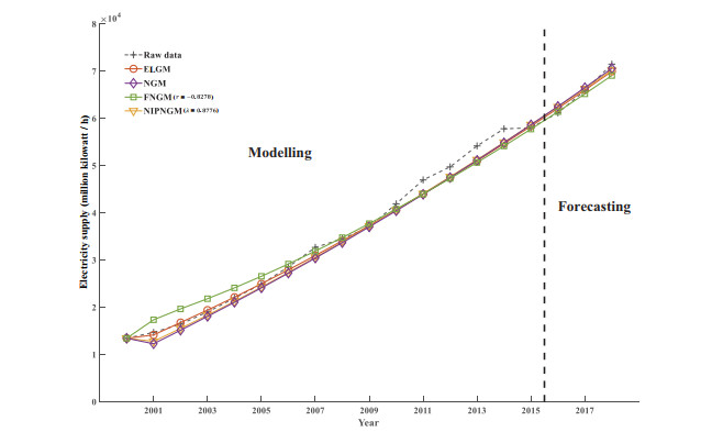
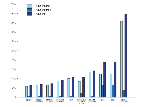
Electricity consumption is one of the most important indicators reflecting the industrialization of a country. Supply of electricity power plays an import role in guaranteeing the running of a country. However, with complex circumstances, it is often difficult to make accurate forecasting with limited reliable data sets. In order to take most advantages of the existing grey system model, the ensemble learning is adopted to provide a new stratagy of building forecasting models for electricity supply of China. The nonhomogeneous grey model with different types of accumulation is firstly fitted with multiple setting of acculumation degrees. Then the majority voting is used to select and combine the most accurate and stable models validated by the grid search cross validation. Two numerical validation cases are taken to validate the proposed method in comparison with other well-known models. Results of the real-world case study of forecasting the electricity supply of China indicate that the proposed model outperforms the other 15 exisiting grey models, which illustrates the proposed model can make much more accurate and stable forecasting in such real-world applications.
Citation: Yubin Cai, Xin Ma. A novel ensemble learning-based grey model for electricity supply forecasting in China[J]. AIMS Mathematics, 2021, 6(11): 12339-12358. doi: 10.3934/math.2021714
Electricity consumption is one of the most important indicators reflecting the industrialization of a country. Supply of electricity power plays an import role in guaranteeing the running of a country. However, with complex circumstances, it is often difficult to make accurate forecasting with limited reliable data sets. In order to take most advantages of the existing grey system model, the ensemble learning is adopted to provide a new stratagy of building forecasting models for electricity supply of China. The nonhomogeneous grey model with different types of accumulation is firstly fitted with multiple setting of acculumation degrees. Then the majority voting is used to select and combine the most accurate and stable models validated by the grid search cross validation. Two numerical validation cases are taken to validate the proposed method in comparison with other well-known models. Results of the real-world case study of forecasting the electricity supply of China indicate that the proposed model outperforms the other 15 exisiting grey models, which illustrates the proposed model can make much more accurate and stable forecasting in such real-world applications.

| [1] | D. C. Li, C. J. Chang, C. C. Chen, W. C. Chen, Forecasting short-term electricity consumption using the adaptive grey-based approach–An Asian case, Omega, 40 (2012), 767–773. |
| [2] | P. F. Pai, W. C. Hong, Support vector machines with simulated annealing algorithms in electricity load forecasting, Energy Convers. Manage., 46 (2005), 2669–2688. |
| [3] | J. Yuan, C. Farnham, C. Azuma, K. Emura, Predictive artificial neural network models to forecast the seasonal hourly electricity consumption for a University Campus, Sustainable Cities Soc., 42 (2018), 82–92. |
| [4] | J. L. Deng, Control problems of grey systems, Syst. Control Lett., 1 (1982), 288–294. |
| [5] | B. Zeng, H. Li, X. Ma, A novel multi-variable grey forecasting model and its application in forecasting the grain production in China, Comput. Ind. Eng., 150 (2020), 106915. |
| [6] | S. Ding, R. Li, Forecasting the sales and stock of electric vehicles using a novel self-adaptive optimized grey model, Eng. Appl. Artif. Intell., 100 (2021), 104148. |
| [7] | W. Wu, X. Ma, Y. Zhang, W. Li, Y. Wang, A novel conformable fractional non-homogeneous grey model for forecasting carbon dioxide emissions of BRICS countries, Sci. Total Environ., 707 (2020), 135447. |
| [8] | Y. Hu, X. Ma, W. Li, W. Wu, D. Tu, Forecasting manufacturing industrial natural gas consumption of China using a novel time-delayed fractional grey model with multiple fractional order, Comput. Appl. Math., 39 (2020), 1–30. |
| [9] | L. Wu, S. Liu, L. Yao, S. Yan, D. Liu, Grey system model with the fractional order accumulation, Commun. Nonlinear Sci. Numer. Simul., 18 (2013), 1775–1785. |
| [10] | W. Zhou, H. Zhang, Y. Dang, Z. Wang, New information priority accumulated grey discrete model and its application, China J. Manage. Sci., 25 (2017), 140–148. |
| [11] | B. Zeng, H. Duan, Y. Zhou, A new multivariable grey prediction model with structure compatibility, Appl. Math. Modell., 75 (2019), 385–397. |
| [12] | X. Ma, W. Wu, B. Zeng, Y. Wang, X. Wu, The conformable fractional grey system model, ISA Trans., 96 (2020), 255–271. |
| [13] | X. Ma, W. Wu, Y. Zhang, Improved GM (1, 1) model based on Simpson formula and its applications, (2019), arXiv: 1908.03493. |
| [14] | B. Wei, N. Xie, A. Hu, Optimal solution for novel grey polynomial prediction model, Appl. Math. Modell., 62 (2018), 717–727. |
| [15] | N. Xie, R. Wang, N. Chen, Measurement of shock effect following change of one-child policy based on grey forecasting approach, Kybernetes, 47 (2018), 559–586. |
| [16] | J. Cui, Y. Dang, S. Liu, Novel grey forecasting model and its modeling mechanism, Control Decis., 24 (2009), 1702–1706. |
| [17] | C. Chen, H. L. Chen, S. P. Chen, Forecasting of foreign exchange rates of Taiwan's major trading partners by novel nonlinear Grey Bernoulli model NGBM (1, 1), Commun. Nonlinear Sci. Numer. Simul., 13 (2008), 1194–1204. |
| [18] | B. Zeng, X. Ma, M. Zhou, A new-structure grey Verhulst model for China's tight gas production forecasting, Appl. Soft Comput., 96 (2020), 106600. |
| [19] | N. Xu, Y. Dang, Y. Gong, Novel grey prediction model with nonlinear optimized time response method for forecasting of electricity consumption in China, Energy, 118 (2017), 473–480. |
| [20] | J. Wang, P. Du, H. Lu, W. Yang, T. Niu, An improved grey model optimized by multi-objective ant lion optimization algorithm for annual electricity consumption forecasting, Appl. Soft Comput., 72 (2018), 321–337. |
| [21] | S. Ding, K. W. Hipel, Y. Dang, Forecasting {China's} electricity consumption using a new grey prediction model, Energy, 149 (2018), 314–328. |
| [22] | C. Liu, W. Wu, W. Xie, J. Zhang, Application of a novel fractional grey prediction model with time power term to predict the electricity consumption of India and China, Chaos Solitons Fractals, 141 (2020), 110429. |
| [23] | L. Yu, X. Ma, W. Wu, X. Xiang, Y. Wang, B. Zeng, Application of a novel time-delayed power-driven grey model to forecast photovoltaic power generation in the Asia-Pacific region, Sustainable Energy Technol. Assess., 44 (2021), 100968. |
| [24] | S. B. Cho, Ensemble of structure-adaptive self-organizing maps for high performance classification, Inf. Sci., 123 (2000), 103–114. |
| [25] | Q. Xiao, C. Li, Y. Tang, L. Li, Meta-reinforcement learning of machining parameters for energy-efficient process control of flexible turning operations, IEEE Trans. Autom. Sci. Eng., 99 (2019), 1–14. |
| [26] | L. Yu, Y. Ma, M. Ma, An effective rolling decomposition-ensemble model for gasoline consumption forecasting, Energy, 222 (2021), 119869. |
| [27] | C. Chen, H. Liu, Dynamic ensemble wind speed prediction model based on hybrid deep reinforcement learning, Adv. Eng. Inf., 48 (2021), 101290. |
| [28] | Z. Dong, J. Liu, B. Liu, K. Li, X. Li, Hourly energy consumption prediction of an office building based on ensemble learning and energy consumption pattern classification, Energy Buildings, 241 (2021), 110929. |
| [29] | C. Y. Lin, Y. S. Chang, S. Abimannan, Ensemble multifeatured deep learning models for air quality forecasting, Atmos. Pollut. Res., 12 (2021), 101045. |
| [30] | A. Vinayagam, V. Veerasamy, P. Radhakrishnan, M. Sepperumal, K. Ramaiyan, An ensemble approach of classification model for detection and classification of power quality disturbances in PV integrated microgrid network, Appl. Soft Comput., 106 (2021), 107294. |
| [31] | X. Ma, M. Xie, J. A. K. Suykens, A novel neural grey system model with Bayesian regularization and its applications, Neurocomputing, 456 (2021), 61–75. |
| [32] | N. Xie, S. Liu, Interval grey number sequence prediction by using non-homogenous exponential discrete grey forecasting model, J. Syst. Eng. Electron., 26 (2015), 96–102. |
| [33] | L. Yu, X. Ma, W. Wu, Y. Wang, B. Zeng, A novel Elastic Net-based NGBMC (1, n) model with multi-objective optimization for nonlinear time series forecasting, Commun. Nonlinear Sci. Numer. Simul., 96 (2021), 105696. |
| [34] | X. Xiang, X. Ma, M. Ma, W. Wu, L. Yu, Research and application of novel Euler polynomial-driven grey model for short-term PM10 forecasting, Grey Syst. Theory Appl., (2020). |
| [35] | L. Liu, L. Wu, Forecasting the renewable energy consumption of the European countries by an adjacent non-homogeneous grey model, Appl. Math. Modell., 89 (2021), 1932–1948. |
| [36] | S. A. Javed, B. Zhu, S. Liu, Forecast of biofuel production and consumption in top CO2 emitting countries using a novel grey model, J. Cleaner Prod., 276 (2020), 123997. |
| [37] | National Bureau of Statistics, Available from: http://www.stats.gov.cn/. |
Figures(6) / Tables(4)

Yubin Cai, Xin Ma. A novel ensemble learning-based grey model for electricity supply forecasting in China[J]. AIMS Mathematics, 2021, 6(11): 12339-12358. doi: 10.3934/math.2021714


 DownLoad: