Extension of TOPSIS method under intuitionistic fuzzy hypersoft environment based on correlation coefficient and aggregation operators to solve decision making problem

Rana Muhammad Zulqarnain; Xiao Long Xin; Muhammad Saeed; Rana Muhammad Zulqarnain; Xiao Long Xin; Muhammad Saeed

doi:10.3934/math.2021167

AIMS Mathematics

2021, Volume 6, Issue 3: 2732-2755. doi: 10.3934/math.2021167

Previous Article Next Article

Research article

Extension of TOPSIS method under intuitionistic fuzzy hypersoft environment based on correlation coefficient and aggregation operators to solve decision making problem

1.
School of Mathematics, Northwest University Xi'an, China
2.
School of Science, Xi'an Polytechnic University, Xi'an 710048, China
3.
Department of Mathematics, School of Science, University of Management and Technology, Lahore, Pakistan

Received: 30 October 2020 Accepted: 20 December 2020 Published: 05 January 2021
MSC : 03E72, 62A86, 68T35, 90B50

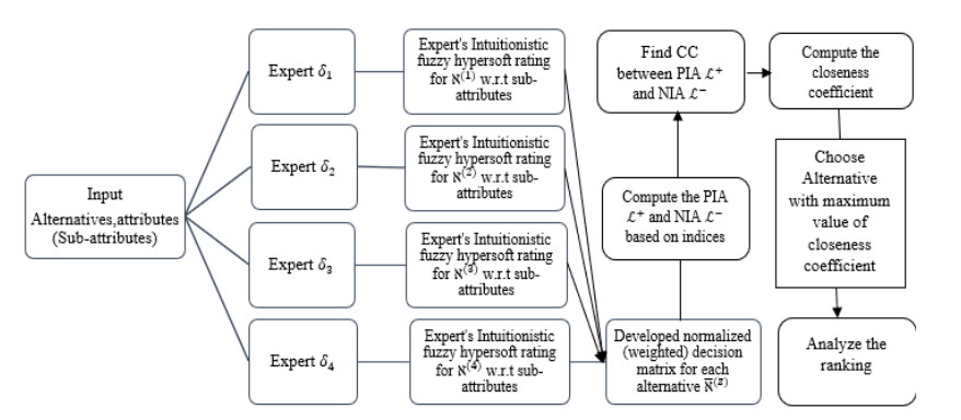
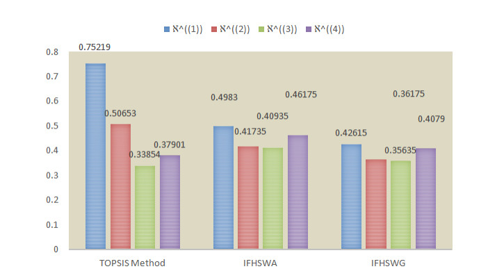
Intuitionistic fuzzy hypersoft set is an extension of the intuitionistic fuzzy soft set used to express insufficient evaluation, uncertainty, and anxiety in decision-making. It is a new technique to realize computational intelligence and decision-making under uncertain conditions. The intuitionistic fuzzy hypersoft set can deal with uncertain and fuzzy information more effectively. The concepts and properties of the correlation coefficient and the weighted correlation coefficient of the intuitionistic fuzzy hypersoft sets are proposed in the following research. A prioritization technique for order preference by similarity to ideal solution (TOPSIS) based on correlation coefficients and weighted correlation coefficients is introduced under the intuitionistic fuzzy hypersoft sets. We also introduced aggregation operators, such as intuitionistic fuzzy hypersoft weighted average and intuitionistic fuzzy hypersoft weighted geometric operators. Based on the established TOPSIS method and aggregation operators, the decision-making algorithm is proposed under an intuitionistic fuzzy hypersoft environment to resolve uncertain and confusing information. A case study on decision-making difficulties proves the application of the proposed algorithm. Finally, a comparative analysis with the advantages, effectiveness, flexibility, and numerous existing studies demonstrates this method's effectiveness.
- hypersoft set,
- intuitionistic fuzzy soft set,
- intuitionistic fuzzy hypersoft set,
- correlation coefficient,
- weighted correlation coefficient,
- TOPSIS
Citation: Rana Muhammad Zulqarnain, Xiao Long Xin, Muhammad Saeed. Extension of TOPSIS method under intuitionistic fuzzy hypersoft environment based on correlation coefficient and aggregation operators to solve decision making problem[J]. AIMS Mathematics, 2021, 6(3): 2732-2755. doi: 10.3934/math.2021167

Related Papers:

Abstract

Intuitionistic fuzzy hypersoft set is an extension of the intuitionistic fuzzy soft set used to express insufficient evaluation, uncertainty, and anxiety in decision-making. It is a new technique to realize computational intelligence and decision-making under uncertain conditions. The intuitionistic fuzzy hypersoft set can deal with uncertain and fuzzy information more effectively. The concepts and properties of the correlation coefficient and the weighted correlation coefficient of the intuitionistic fuzzy hypersoft sets are proposed in the following research. A prioritization technique for order preference by similarity to ideal solution (TOPSIS) based on correlation coefficients and weighted correlation coefficients is introduced under the intuitionistic fuzzy hypersoft sets. We also introduced aggregation operators, such as intuitionistic fuzzy hypersoft weighted average and intuitionistic fuzzy hypersoft weighted geometric operators. Based on the established TOPSIS method and aggregation operators, the decision-making algorithm is proposed under an intuitionistic fuzzy hypersoft environment to resolve uncertain and confusing information. A case study on decision-making difficulties proves the application of the proposed algorithm. Finally, a comparative analysis with the advantages, effectiveness, flexibility, and numerous existing studies demonstrates this method's effectiveness.

References

[1]	L. A. Zadeh, Fuzzy Sets, Information and Control, 8 (1965), 338–353.
[2]	K. Atanassov, Intuitionistic Fuzzy Sets, Fuzzy Set. Syst., 20 (1986), 87–96.
[3]	H. Garg, G. Kaur, Cubic intuitionistic fuzzy sets and its fundamental properties, J. Mult-valued Log. S., 33 (2019), 507–537.
[4]	K. Atanassov, G. Gargov, Interval valued intuitionistic fuzzy sets, Fuzzy Set. Syst., 31 (1989), 343–349. doi: 10.1016/0165-0114(89)90205-4
[5]	H. Garg, K. Kumar, Linguistic interval-valued Atanassov intuitionistic fuzzy sets and their applications to group decision-making problems, IEEE T. Fuzzy Syst., 27 (2019), 2302–2311. doi: 10.1109/TFUZZ.2019.2897961
[6]	J. C. R. Alcantud, A. Z. Khameneh, A. Kilicman, Aggregation of infinite chains of intuitionistic fuzzy sets and their application to choices with temporal intuitionistic fuzzy information, Information Sciences, 514 (2020), 106–117. doi: 10.1016/j.ins.2019.12.008
[7]	D. Molodtsov, Soft set theory-First results, Comput. Math. Appl., 37 (1999), 19–31.
[8]	P. K. Maji, R. Biswas, A. R. Roy, Fuzzy soft sets, Journal of Fuzzy Mathematics, 9 (2001), 589–602.
[9]	G. Ali, M. Akram, A. N. A. Koam, J. C. R. Alcantud, Parameter Reductions of Bipolar Fuzzy Soft Sets with Their Decision-Making Algorithms, Symmetry, 11 (2019), 1–25.
[10]	P. Maji, R. Biswas, A. Roy, Intuitionistic fuzzy soft sets, Journal of Fuzzy Mathematics, 9 (2001), 677–692.
[11]	X. Yang, T. Y. Lin, J. Yang, Y. Li, D. Yu, Combination of interval-valued fuzzy set and soft set, Comput. Math. Appl., 58 (2009), 521–527. doi: 10.1016/j.camwa.2009.04.019
[12]	M. Akram, G. Ali, J. C. R. Alcantud, New decision-making hybrid model: intuitionistic fuzzy N-soft rough sets, Soft Comput., 23 (2019), 9853–9868. doi: 10.1007/s00500-019-03903-w
[13]	T. Gerstenkorn, J. Mafiko, Correlation of intuitionistic fuzzy sets, Fuzzy Set. Syst., 44 (1991), 39–43. doi: 10.1016/0165-0114(91)90031-K
[14]	C. Yu, Correlation of fuzzy numbers, Fuzzy Set. Syst., 55 (1993), 303–307.
[15]	D. A. Chiang, N. P. Lin, Correlation of fuzzy sets, Fuzzy Set. Syst., 102 (1999), 221–226.
[16]	H. Garg, An improved cosine similarity measure for intuitionistic fuzzy sets and their applications to decision-making process, Hacet. J. Math. Stat., 47 (2018), 1578–1594.
[17]	H. Garg, K. Kumar, An advanced study on the similarity measures of intuitionistic fuzzy sets based on the set pair analysis theory and their application in decision making, Soft Comput., 22 (2018), 4959–4970. doi: 10.1007/s00500-018-3202-1
[18]	H. Garg, D. Rani, A robust correlation coefficient measure of complex intuitionistic fuzzy sets and their applications in decision-making, Appl. Intell., 49 (2018), 496–512.
[19]	W. L. Hung, J. W. Wu, Correlation of intuitionistic fuzzy sets by centroid method, Information Sciences., 144 (2002), 219–225. doi: 10.1016/S0020-0255(02)00181-0
[20]	H. Bustince, P. Burillo, Correlation of interval-valued intuitionistic fuzzy sets, Fuzzy Set. Syst., 74 (1995), 237–244. doi: 10.1016/0165-0114(94)00343-6
[21]	D. H. Hong, A note on correlation of interval-valued intuitionistic fuzzy sets, Fuzzy Set. Syst., 95 (1998), 113–117. doi: 10.1016/S0165-0114(96)00311-9
[22]	H. B. Mitchell, A correlation coefficient for intuitionistic fuzzy sets, Int. J. Intell. Syst., 19 (2004), 483–490. doi: 10.1002/int.20004
[23]	H. Garg, R. Arora, TOPSIS method based on correlation coefficient for solving decision-making problems with intuitionistic fuzzy soft set information, AIMS Mathematics, 5 (2020), 2944–2966. doi: 10.3934/math.2020190
[24]	H. L. Huang, Y. Guo, An Improved Correlation Coefficient of Intuitionistic Fuzzy Sets, J. Intell. Syst., 28 (2019), 231–243. doi: 10.1515/jisys-2017-0094
[25]	S. Singh, S. Sharma, S. Lalotra, Generalized Correlation Coefficients of Intuitionistic Fuzzy Sets with Application to MAGDM and Clustering Analysis, Int. J. Fuzzy Syst., 22 (2020), 1582–1595. doi: 10.1007/s40815-020-00866-1
[26]	C. L. Hwang, K. Yoon, Multiple Attribute Decision Making Methods and Applications, Lecture Notes in Economics and Mathematical Systems, Springer-Verlag Berlin Heidelberg, 1981.
[27]	M. Zulqarnain, F. Dayan, M. Saeed, TOPSIS Analysis for The Prediction of Diabetes Based on General Characteristics of Humans, International Journal of Pharmaceutical Sciences and Research, 9 (2018), 2932–2939.
[28]	A. Sarkar, A TOPSIS method to evaluate the technologies, International Journal of Quality & Reliability Management, 31 (2013), 2–13.
[29]	R. M. Zulqarnain, S. Abdal, B. Ali, L. Ali, F. Dayan, M. I. Ahamad, et al. Selection of Medical Clinic for Disease Diagnosis by Using TOPSIS Method, International Journal of Pharmaceutical Sciences Review and Research, 61 (2020), 22–27.
[30]	C. T. Chen, Extensions of the TOPSIS for group decision-making under fuzzy environment, Fuzzy Set. Syst., 114 (2000), 1–9. doi: 10.1016/S0165-0114(97)00377-1
[31]	L. Dymova, P. Sevastjanov, A. Tikhonenko, An approach to generalization of fuzzy TOPSIS method, Information Sciences, 238 (2013), 149–162. doi: 10.1016/j.ins.2013.02.049
[32]	M. Zulqarnain, F. Dayan, Choose Best Criteria for Decision Making Via Fuzzy Topsis Method, Mathematics and Computer Science, 2 (2017), 113–119. doi: 10.11648/j.mcs.20170206.14
[33]	A. Y. Yayla, A. Özbek, A. Yildiz, Fuzzy TOPSIS method in supplier selection and application in the garment industry, Fibres Text. East.Eur., 20 (2012), 20–23.
[34]	M. Zulqarnain, F. Dayan, Selection Of Best Alternative For An Automotive Company By Intuitionistic Fuzzy TOPSIS Method, International journal of scientific & technology research, 6 (2017), 126–132.
[35]	M. Akram, A. Adeel, J. C. R. Alcantud, Multi-Criteria Group Decision-Making Using an m-Polar Hesitant Fuzzy TOPSIS Approach, Symmetry, 11 (2019), 1–23.
[36]	H. Garg, R. Arora, Generalized and group-based generalized intuitionistic fuzzy soft sets with applications in decision-making, Appl. Intell., 48 (2018), 343–356. doi: 10.1007/s10489-017-0981-5
[37]	K. Zhang, J. Zhan, X. Wang, TOPSIS-WAA method based on a covering-based fuzzy rough set: an application to rating problem, Information Sciences, 539 (2020), 397–421. doi: 10.1016/j.ins.2020.06.009
[38]	H. Jiang, J. Zhan, B. Sun, J. C. R. Alcantud, An MADM approach to covering-based variable precision fuzzy rough sets: an application to medical diagnosis, Int. J. Mach. Learn. Cyb., 11 (2020), 2181–2207. doi: 10.1007/s13042-020-01109-3
[39]	T. Mahmood, Z. Ali, Entropy measure and TOPSIS method based on correlation coefficient using complex q-rung orthopair fuzzy information and its application to multi-attribute decision making, Soft Comput., 11 (2020), 1–27. doi: 10.5121/ijsc.2020.11401
[40]	J. Zhan, H. Jiang, Y. Yao, Covering-based variable precision fuzzy rough sets with PROMETHEE-EDAS methods, Information Sciences, 538 (2020), 314–336. doi: 10.1016/j.ins.2020.06.006
[41]	J. Ye, J. Zhan, Z. Xu, A novel decision-making approach based on three-way decisions in fuzzy information systems, Information Sciences, 541 (2020), 362–390. doi: 10.1016/j.ins.2020.06.050
[42]	J. Zhan, H. Jiang, Y. Yao, Three-way multi-attribute decision-making based on outranking relations, IEEE T. Fuzzy Syst., 2020, DOI: 10.1109/TFUZZ.2020.3007423.
[43]	L. Zhang, J. Zhan, Y. Yao, Intuitionistic fuzzy TOPSIS method based on CVPIFRS models: an application to biomedical problems, Information Sciences, 517 (2020), 315–339. doi: 10.1016/j.ins.2020.01.003
[44]	J. Zhan, B. Sun, Covering-based intuitionistic fuzzy rough sets and applications in multi-attribute decision-making, Artif. Intell. Re., 53 (2020), 671–701. doi: 10.1007/s10462-018-9674-7
[45]	F. Smarandache, Extension of Soft Set to Hypersoft Set, and then to Plithogenic Hypersoft Set, Neutrosophic Sets and Systems, 22 (2018), 168–170.
[46]	S. Rana, M. Qayyum, M. Saeed, F. Smarandache, Plithogenic Fuzzy Whole Hypersoft Set: Construction of Operators and their Application in Frequency Matrix Multi Attribute Decision Making Technique, Neutrosophic Sets and Systems, 28 (2019), 34–50.
[47]	R. M. Zulqarnain, X. L. Xin, M. Saqlain, F. Smarandache, Generalized Aggregate Operators on Neutrosophic Hypersoft Set, Neutrosophic Sets and Systems, 36 (2020), 271–281.
[48]	S. Alkhazaleh, Plithogenic Soft Set, Neutrosophic Sets and Systems, 33 (2020), 256–274.
[49]	M. Abdel-Basset, W. Ding, R. Mohamed, N. Metawa, An integrated plithogenic MCDM approach for financial performance evaluation of manufacturing industries, Risk Manag., 22 (2020), 192–218. doi: 10.1057/s41283-020-00061-4
[50]	M. Abdel-Basset, R. Mohamed, A. E. N. H. Zaied, F. Smarandache, A Hybrid Plithogenic Decision-Making Approach with Quality Function Deployment for Selecting Supply Chain Sustainability Metrics, Symmetry, 11 (2019), 1–21.
[51]	R. Arora, H. Garg, Robust aggregation operators for multi-criteria decision-making with intuitionistic fuzzy soft set environment, Sci. Iran., 25 (2018), 931–942.
[52]	Z. Xu, J. Chen, J. Wu, Clustering algorithm for intuitionistic fuzzy sets, Information Sciences, 178 (2008), 3775–3790. doi: 10.1016/j.ins.2008.06.008
[53]	H. M. Zhang, Z. S. Xu, Q. Chen, On clustering approach to intuitionistic fuzzy sets, Control and Decision, 22 (2007), 882–888.

Reader Comments

Your name:*

Email:*
© 2021 the Author(s), licensee AIMS Press. This is an open access article distributed under the terms of the Creative Commons Attribution License (http://creativecommons.org/licenses/by/4.0)