The restoration mechanism (RM) and subgrain characteristics of 0.05C-1.52Cu-1.51Mn steel in single-hit plane strain compression (PSC) were investigated using a thermomechanical simulator (Gleeble). It was observed that at diminished deformation temperature (DT) and larger strain rate, the austenitic phase (during deformation) showed some thermal/dynamic softening (TH/DRS), but it did not reach the condition where the "work hardening rate" (WH rate)became constant with the stress, i.e., dynamic recovery (DRV) softening balances work hardening (WH). However, it was observed that at higher DT and lower strain rate, the "WH rate" for samples deformed at 850 ℃ (at a strain rate of 0.01 s−1), 950 ℃ (at strain rates of 0.1 and 0.01 s−1) and 1000 ℃ (at strain rates of 0.1 and 0.01 s−1) increased to negative peak, and then decreased to almost zero (for samples deformed at 950 and 1000 ℃ at a strain rate of 0.01 s−1), which is the onset of steady-state flow. When the sample deformed at 750 ℃ followed by quenching, the microstructure was indicative of a deformed microstructure rather than a transformed microstructure. It was observed that there was an increase in the extent of substructure formation and a decrease in mean subgrain size with increasing strain rate. When samples deformed at 850,950 and 1000 ℃, these temperature ranges were above Ar3 temperature. Hence quenching would lead to a phase transformation and hence the deformed microstructure would be eliminated. The room temperature microstructures when the sample deformed at a strain rate of 1 s−1, were nicely equiaxed and clean with no dislocations present. However, at lower strain rates of 0.1 and 0.01 s−1, microstructure showed substructures.
Citation: Pawan Kumar. Subgrain characterization of low carbon copper bearing steel under plane strain compression using electron backscattered diffraction[J]. AIMS Materials Science, 2023, 10(6): 1121-1143. doi: 10.3934/matersci.2023060
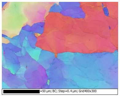
The restoration mechanism (RM) and subgrain characteristics of 0.05C-1.52Cu-1.51Mn steel in single-hit plane strain compression (PSC) were investigated using a thermomechanical simulator (Gleeble). It was observed that at diminished deformation temperature (DT) and larger strain rate, the austenitic phase (during deformation) showed some thermal/dynamic softening (TH/DRS), but it did not reach the condition where the "work hardening rate" (WH rate)became constant with the stress, i.e., dynamic recovery (DRV) softening balances work hardening (WH). However, it was observed that at higher DT and lower strain rate, the "WH rate" for samples deformed at 850 ℃ (at a strain rate of 0.01 s−1), 950 ℃ (at strain rates of 0.1 and 0.01 s−1) and 1000 ℃ (at strain rates of 0.1 and 0.01 s−1) increased to negative peak, and then decreased to almost zero (for samples deformed at 950 and 1000 ℃ at a strain rate of 0.01 s−1), which is the onset of steady-state flow. When the sample deformed at 750 ℃ followed by quenching, the microstructure was indicative of a deformed microstructure rather than a transformed microstructure. It was observed that there was an increase in the extent of substructure formation and a decrease in mean subgrain size with increasing strain rate. When samples deformed at 850,950 and 1000 ℃, these temperature ranges were above Ar3 temperature. Hence quenching would lead to a phase transformation and hence the deformed microstructure would be eliminated. The room temperature microstructures when the sample deformed at a strain rate of 1 s−1, were nicely equiaxed and clean with no dislocations present. However, at lower strain rates of 0.1 and 0.01 s−1, microstructure showed substructures.

| [1] |
Makhatha ME (2022) Effect of titanium addition on sub-structural characteristics of low carbon copper bearing steel in hot rolling. AIMS Mater Sci 9: 604–616. https://www.aimspress.com/article/doi/10.3934/matersci.2022036 doi: 10.3934/matersci.2022036

|
| [2] |
Sakai T, Belyakov A, Kaibyshev R, et al. (2014) Dynamic and post-dynamic recrystallization under hot, cold and severe plastic deformation conditions. Prog Mater Sci 60: 130–207. https://doi.org/10.1016/j.pmatsci.2013.09.002 doi: 10.1016/j.pmatsci.2013.09.002
|
| [3] | Link TM, Hance BM (2003) Effects of strain rate and temperature on the work hardening behavior of high strength sheet steels. SAE Trans 112: 211–219. http://www.jstor.org/stable/44699575 |
| [4] |
Sakai T, Jonas JJ (1984) Overview no. 35 Dynamic recrystallization: Mechanical and microstructural considerations. Acta Metall 32: 189–209. https://doi.org/10.1016/0001-6160(84)90049-X doi: 10.1016/0001-6160(84)90049-X
|
| [5] |
Gourdet S, Montheillet F (2000) An experimental study of the recrystallization mechanism during hot deformation of aluminium. Mater Sci Eng A 283: 274–288. https://doi.org/10.1016/S0921-5093(00)00733-4 doi: 10.1016/S0921-5093(00)00733-4
|
| [6] |
Belyakov A, Tsuzaki K, Miura H, et al. (2003) Effect of initial microstructures on grain refinement in a stainless steel by large strain deformation. Acta Mater 51: 847–861. https://doi.org/10.1016/S1359-6454(02)00476-7 doi: 10.1016/S1359-6454(02)00476-7
|
| [7] |
Solberg JK, McQueen HJ, Ryum N, et al. (1989) Influence of ultra-high strains at elevated temperatures on the microstructure of aluminium. Philos Mag A 60: 447–471. https://doi.org/10.1080/01418618908213872 doi: 10.1080/01418618908213872
|
| [8] |
Hales SJ, McNelley TR, McQueen HJ (1991) Recrystallization and superplasticity at 300 ℃ in an aluminum-magnesium alloy. Metall Trans A 22: 1037–1047. https://doi.org/10.1007/BF02661097 doi: 10.1007/BF02661097
|
| [9] |
Tsuji N, Matsubara Y, Saito Y (1997) Dynamic recrystallization of ferrite in interstitial free steel. Scripta Mater 37: 477–484. https://doi.org/10.1016/S1359-6462(97)00123-1 doi: 10.1016/S1359-6462(97)00123-1
|
| [10] |
McNelley TR, McMahon ME (1997) Microtexture and grain boundary evolution during microstructural refinement processes in SUPRAL 2004. Metall Mater Trans A 28: 1879–1887. https://doi.org/10.1007/s11661-997-0118-2 doi: 10.1007/s11661-997-0118-2
|
| [11] |
Jorge AM, Balancin O (2005) Prediction of steel flow stresses under hot working conditions. Mat Res 8: 309–315. https://doi.org/10.1590/S1516-14392005000300015 doi: 10.1590/S1516-14392005000300015
|
| [12] |
Kingkam W, Li N, Zhang HX, et al. (2017) Hot deformation behavior of high strength low alloy steel by thermo mechanical simulator and finite element method. IOP Conf Ser Mater Sci Eng 205: 012001. https://dx.doi.org/10.1088/1757-899X/205/1/012001 doi: 10.1088/1757-899X/205/1/012001
|
| [13] |
Doherty RD, Hughes DA, Humphreys FJ, et al. (1997) Current issues in recrystallization: A review. Mater Sci Eng A 238: 219–274. https://doi.org/10.1016/S0921-5093(97)00424-3 doi: 10.1016/S0921-5093(97)00424-3
|
| [14] |
Quan GZ, Wang Y, Liu YY, et al. (2013) Effect of temperatures and strain rates on the average size of grains refined by dynamic recrystallization for as-extruded 42CrMo steel. Mat Res 16: 1092–1105. https://doi.org/10.1590/S1516-14392013005000091 doi: 10.1590/S1516-14392013005000091
|
| [15] |
Kumar P, Hodgson P, Beladi H, et al. (2020) EBSD investigation to study the restoration mechanism and substructural characteristics of 23Cr-6Ni-3Mo duplex stainless steel during post-deformation annealing. Trans Indian Inst Met 73: 1421–1431. https://doi.org/10.1007/s12666-020-01884-1 doi: 10.1007/s12666-020-01884-1
|
| [16] |
Montheillet F, Jonas JJ (1996) Temperature dependence of the rate sensitivity and its effect on the activation energy for high-temperature flow. Metall Mater Trans A 27: 3346–3348. https://doi.org/10.1007/BF02663887 doi: 10.1007/BF02663887
|
| [17] |
Davenport SB, Silk NJ, Sparks CN, et al. (2000) Development of constitutive equations for modelling of hot rolling. Mater Sci Technol 16: 539–546. https://doi.org/10.1179/026708300101508045 doi: 10.1179/026708300101508045
|
| [18] |
Sarkar A, Chakravartty JK (2013) Investigation of progress in dynamic recrystallization in two austenitic stainless steels exhibiting flow softening. J Metall Eng 2: 130–136. https://doi.org/10.5923/j.ijmee.20130202.03 doi: 10.5923/j.ijmee.20130202.03
|
| [19] |
Sarkar A, Kapoor R, Verma A, et al. (2012) Hot deformation behavior of Nb-1Zr-0.1C alloy in the temperature range 700–1700 ℃. J Nucl Mater 422: 1–7. https://doi.org/10.1016/j.jnucmat.2011.11.064 doi: 10.1016/j.jnucmat.2011.11.064
|
| [20] |
De Oliveira TS, Silva ES, Rodrigues SF, et al. (2017) Softening mechanisms of the AISI 410 martensitic stainless steel under hot torsion simulation. Mat Res 20: 395–406. https://doi.org/10.1590/1980-5373-MR-2016-0795 doi: 10.1590/1980-5373-mr-2016-0795
|
| [21] |
Prasad YVRK, Ravichandran N (1991) Effect of stacking fault energy on the dynamic recrystallization during hot working of FCC metals: A study using processing maps. Bull Mater Sci 14: 1241–1248. https://doi.org/10.1007/BF02744618 doi: 10.1007/BF02744618
|
| [22] |
Kumar P, Hodgson P, Beladi H, et al. (2021) Restoration mechanism and sub-structural characteristics of duplex stainless steel with an initial equiaxed austenite morphology during post-deformation annealing. Key Eng Mater 882: 64–73. https://doi.org/10.4028/www.scientific.net/KEM.882.64 doi: 10.4028/www.scientific.net/KEM.882.64
|


Figures(32) / Tables(2)

Pawan Kumar. Subgrain characterization of low carbon copper bearing steel under plane strain compression using electron backscattered diffraction[J]. AIMS Materials Science, 2023, 10(6): 1121-1143. doi: 10.3934/matersci.2023060


 DownLoad: