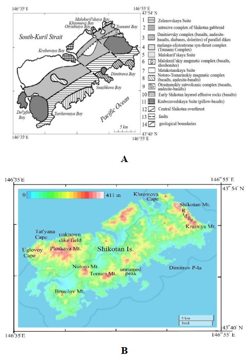
In this paper, for the first time, we used Google Earth, an easily accessible method for obtaining geological information to study Shikotan Island (Lesser Kuril Arc). Google Earth flight mode made it possible to examine coastal cliffs on the island, which are inaccessible for hiking or walking, whereas 3-D visualization mode helped us study topographic features, tectonic dislocations, and sediment layering hidden by vegetation and soil, thereby significantly expanding understanding of the geologic structure of the island. Researchers conducting studies in the northwestern part of the island (Tat'yana Cape) discovered a previously unknown structure—a dike field. In the southern part, two thrust faults were identified: An unnamed peak and Tomari Mountain, previously considered a volcano. In the southwestern part of Shikotan Island, there are four unknown volcanic peaks. Together with the Notoro Volcano, they mark the rim of an interpreted caldera of a paleovolcano, which could have been the main unknown source of tuffaceous material for the Mesozoic-Cenozoic deposits of the Matakotanskaya, Malokuril'skaya, and Zelenovskaya Suites. It has been shown that the gabbroid massif of Tsunami Bay (northeastern part of the island) is an autochthonous (local) formation, and not allochthonous, that is, brought from the Pacific Ocean, as evidenced by an intrusive contact with the rocks of the Malokuril'skaya Suite. Despite these positive results, analysis of satellite images of Shikotan Island unexpectedly has not confirmed the existence of the Central Shikotan thrust fault, the largest previously mapped tectonic structure on the island. This work confirms that Google Earth is a very useful tool for geological research in remote areas.
Citation: Evgeny P Terekhov, Anatoly V Mozherovsky. Some features of geological structure of the Shikotan Island (Lesser Kuril Arc)—A view from 'Space'[J]. AIMS Geosciences, 2024, 10(4): 907-917. doi: 10.3934/geosci.2024042
In this paper, for the first time, we used Google Earth, an easily accessible method for obtaining geological information to study Shikotan Island (Lesser Kuril Arc). Google Earth flight mode made it possible to examine coastal cliffs on the island, which are inaccessible for hiking or walking, whereas 3-D visualization mode helped us study topographic features, tectonic dislocations, and sediment layering hidden by vegetation and soil, thereby significantly expanding understanding of the geologic structure of the island. Researchers conducting studies in the northwestern part of the island (Tat'yana Cape) discovered a previously unknown structure—a dike field. In the southern part, two thrust faults were identified: An unnamed peak and Tomari Mountain, previously considered a volcano. In the southwestern part of Shikotan Island, there are four unknown volcanic peaks. Together with the Notoro Volcano, they mark the rim of an interpreted caldera of a paleovolcano, which could have been the main unknown source of tuffaceous material for the Mesozoic-Cenozoic deposits of the Matakotanskaya, Malokuril'skaya, and Zelenovskaya Suites. It has been shown that the gabbroid massif of Tsunami Bay (northeastern part of the island) is an autochthonous (local) formation, and not allochthonous, that is, brought from the Pacific Ocean, as evidenced by an intrusive contact with the rocks of the Malokuril'skaya Suite. Despite these positive results, analysis of satellite images of Shikotan Island unexpectedly has not confirmed the existence of the Central Shikotan thrust fault, the largest previously mapped tectonic structure on the island. This work confirms that Google Earth is a very useful tool for geological research in remote areas.

| [1] | Govorov G (2000) Geodynamics of Small-Kuril paleoarc system after geochronological and petrochemical data. Dokl Earth Sci 372: 521–524. In Russian. |
| [2] | Govorov G (2002) Phanerozoic Magmatic Belts and Origin of the Okhotsk Sea Geoblock Structure. Dalnauka Vladivostok: 1–97. In Russian. |
| [3] | Parfenov L, Popeko V, Popeko L (1983) The main structural and material complexes of Shikotan Island and their geological nature (Lesser Kurile Islands). Russ Geol Geophys 10: 24–34. In Russian. |
| [4] | Melankholina EN (1978) Gabbroids and parallel dikes in the structure of the island of Shikotan (Lesser Kuril Islands). Geotectonics. 3: 128–136. |
| [5] | Gorshkov G, Markhinin E, Rodionova R, et al. (1964) Description of the volcanoes of the Kuril Islands. Geol USSR 31: 581–604. In Russian. |
| [6] | Sasa Y (1932) On the geological structure of Shikotan Island (Lesser Kuril Ridge). Geol J 39: 465. In Russian. |
| [7] | Goliokko B (1992) The structure and geological development of the southern part of the Kuril island arc in the Late Cretaceous-Miocene in connection with the subduction of the Pacific plate. Dissertation, Shirshov Institute of Oceanology of Russian Academy of Sciences. In Russian. |
| [8] | Bogatikov O, Tsvetkov A (1988) Magmatic Evolution of Island Arcs, Nauka, Moscow, 1–247. In Russian. |
| [9] | Frolova T, Burikova I, Guschin A, et al. (1985) The Origin of the Volcanic Series of Island Arcs, Nedra, Moscow, 275. In Russian. |
| [10] | Frolova T, Burikova I, Frolov V, et al. (1977) Peculiarities of volcanism of the Lesser Kuril Arc. Bulletin MOIP Branch of the Geology 4: 38–50. In Russian. |
| [11] | Govorov G, Tsvetkov A (1985) Basaltoid magmatism of the Lesser Kuril Arc, In: Volcanic and Volcanic-Sedimentary Rocks of the Far East, Far Eastern Branch of the USSR Academy of Sciences, Vladivostok. In Russian. |
| [12] | Krasilov V, Blohina N, Kundyshev A, et al. (1986) New data on the stratigraphy and geological history of the Lesser Kuril Arc. Dokl Earth Sci 291: 177–180. In Russian. |
| [13] | Terekhov E, Mozherovsky A (2007) Bottom relief of the central part of the Sea of Okhotsk (View from space). Dep. VINITI 327-В2007. Available from: https://elibrary.ru/item.asp?id = 18282357. In Russian. |
| [14] |
Markevich VS, Mozherovsky AV, Terekhov EP (2012) Palynological characteristics of the sediments of the Malokuril'skaya formation (Maastrichtian-Danian), Shikotan Island. Stratigr Geol Correl 20: 466–477. https://doi.org/10.1134/S0869593812040041 doi: 10.1134/S0869593812040041

|
| [15] | Mozherovsky AV, Terekhov EP (2016) Authigenic minerals of Meso-Cenozoic volcanic-sedimentary rocks of marginal seas bottom of the North-Western Pacific. Stand Glob J Geol Explor Res 3: 105–114. |
| [16] |
Palechek TN, Terekhov EP, Mozherovskii AV (2008) Campanian-Maastrichtian radiolarians from the Malokuril'skaya formation, the Shikotan Island. Stratigr Geol Correl 16: 650–663. https://doi.org/10.1134/S0869593808060051 doi: 10.1134/S0869593808060051
|
| [17] |
Tsvetkov AA, Govorov GI, Tsvetkova MV, et al. (1986) The Evolution of Magmatism in the Lesser Kuril Ridge of the Kuril Island-Arc System. Int Geol Rev 28: 180–196. https://doi.org/10.1080/00206818609466259 doi: 10.1080/00206818609466259
|


Figures(7)

Evgeny P Terekhov, Anatoly V Mozherovsky. Some features of geological structure of the Shikotan Island (Lesser Kuril Arc)—A view from "Space"[J]. AIMS Geosciences, 2024, 10(4): 907-917. doi: 10.3934/geosci.2024042


 DownLoad: