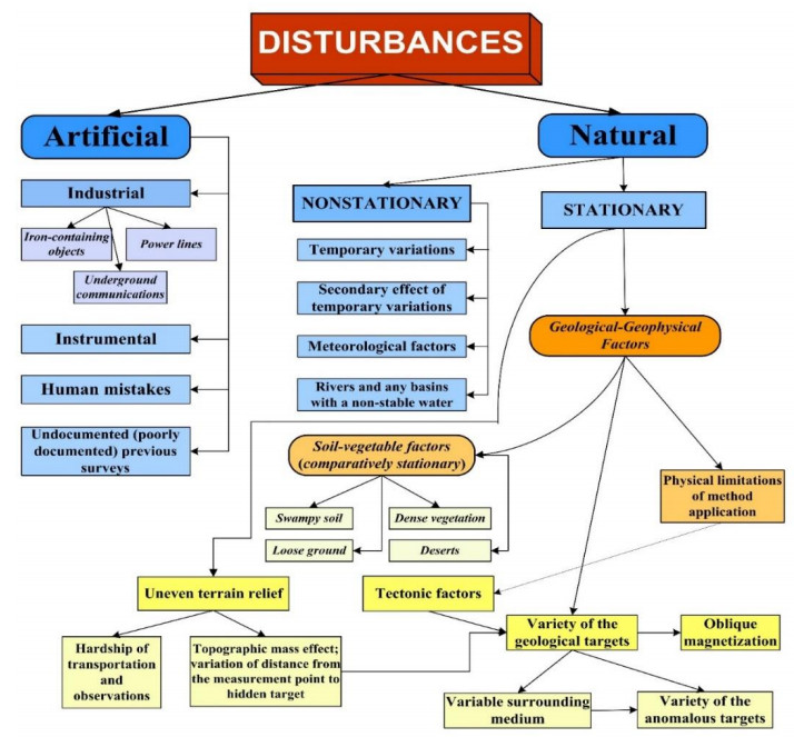
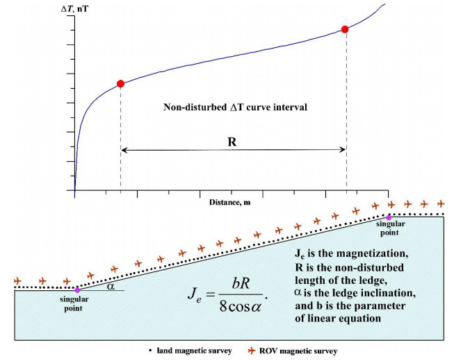
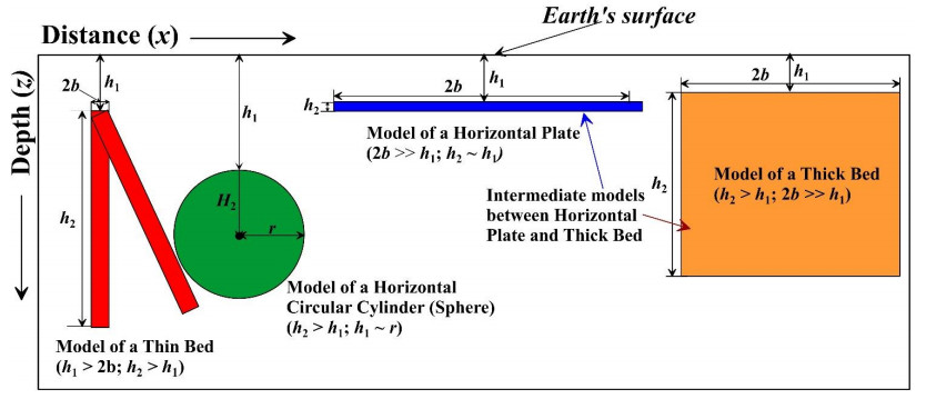
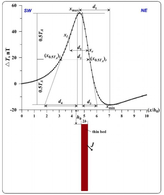
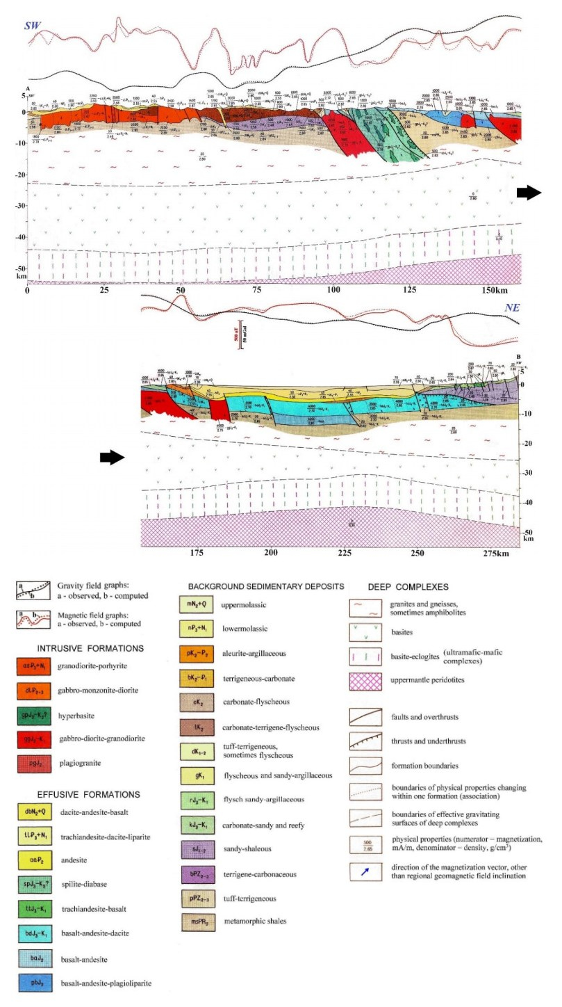
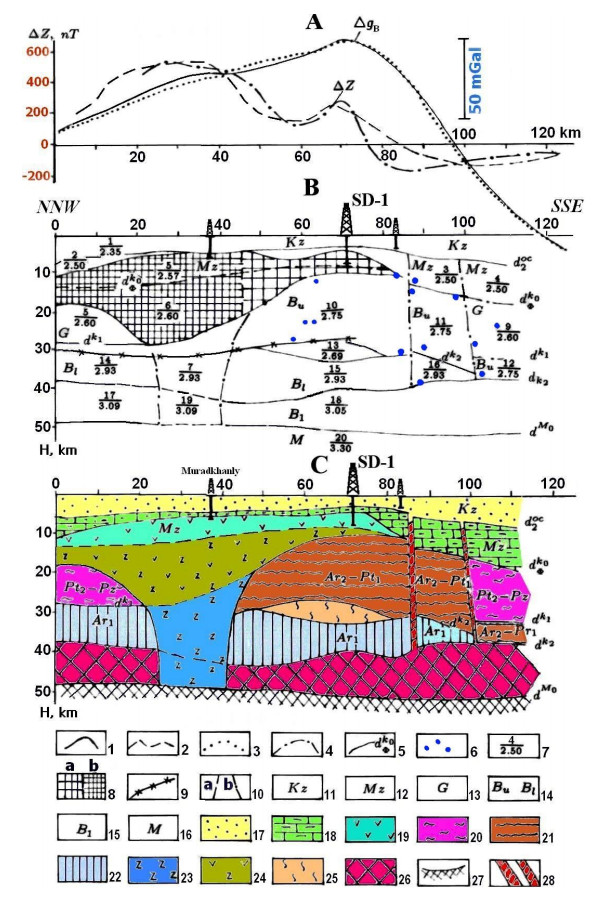
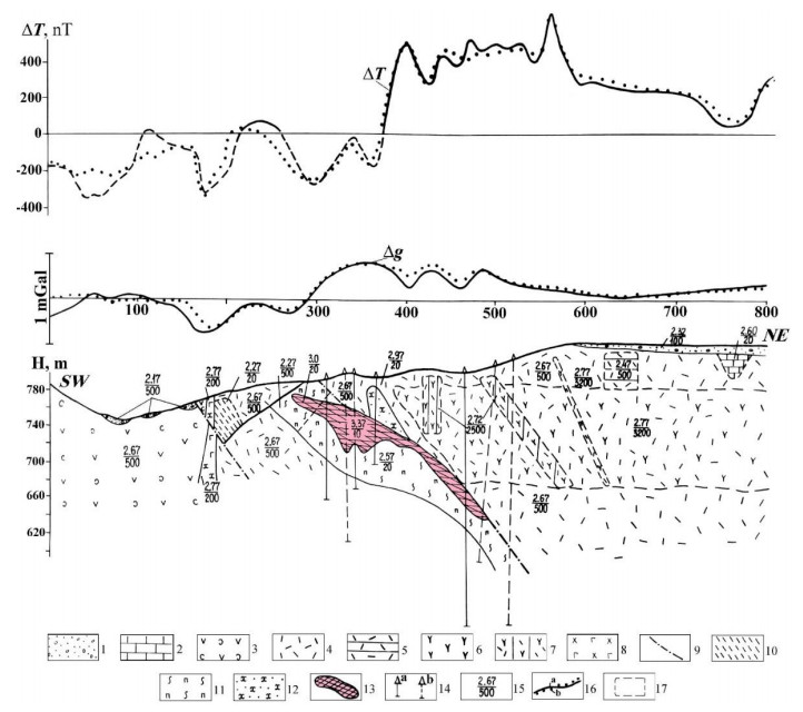
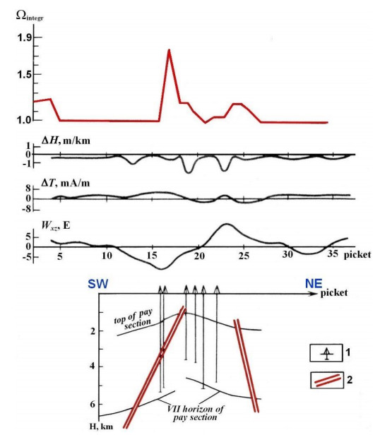
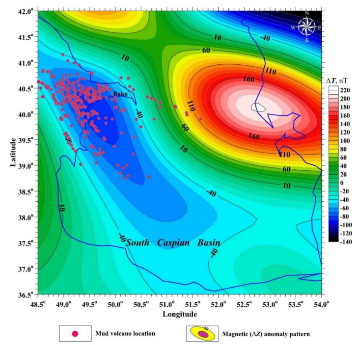
With the rapid development of aeromagnetic (primarily uncrewed) methods for measuring the magnetic field, the possibility of detailed magnetic research in hard-to-reach mountainous areas, forested areas, swamp areas, desert areas, and water areas has emerged. The conditions for interpreting the magnetic field are most difficult due to the vector nature of the magnetic properties of rocks, the wide range of their properties, and the presence of residual magnetization. The physical and geological conditions of the territory of Azerbaijan are characterized by rugged terrain relief, inclined magnetization (~58°), and complex geological environments. Along with using a probabilistic approach, deterministic methods for solving inverse and direct problems of geophysics become of great importance since it is possible to identify relatively extended reference boundaries and analyze magnetic anomalies from separate bodies of relatively simple shape. The article briefly outlines the main stages of processing and interpreting magnetic data under complex environments. The theoretical examples discussed include a block diagram of various disturbances, interpretive models of thin and thick beds, an intermediate model, a thin horizontal plate, and a horizontal circular cylinder on the flat and inclined surfaces under inclined magnetization conditions. The process of assessing magnetization on sloping terrain relief is shown. The presented field examples for the Caucasus Mountains show the quantitative interpretation of aeromagnetic data at the Big Somalit and Guton sites (southern Greater Caucasus, Azerbaijan), a deep regional profile through the Lesser and Greater Caucasus, magnetic field studies in the area around the Saatly superdeep borehole (Middle Kur depression between the Greater and Lesser Caucasus), and 3D magnetic field modeling at the Gyzylbulag gold deposit (the Azerbaijani part of the Lesser Caucasus). In the Caspian Sea, we demonstrated the use of an information parameter to identify faults in the Bulla hydrocarbon field (Gulf of Baku) and, for the first time, obtained the relationship between the generalized aeromagnetic data (2.5 kilometers over the mean sea level) and the central area of the mud volcanoes distribution in Azerbaijan.
Citation: Lev Eppelbaum. Processing and interpretation of magnetic data in the Caucasus Mountains and the Caspian Sea: A review[J]. AIMS Geosciences, 2024, 10(2): 333-370. doi: 10.3934/geosci.2024019
With the rapid development of aeromagnetic (primarily uncrewed) methods for measuring the magnetic field, the possibility of detailed magnetic research in hard-to-reach mountainous areas, forested areas, swamp areas, desert areas, and water areas has emerged. The conditions for interpreting the magnetic field are most difficult due to the vector nature of the magnetic properties of rocks, the wide range of their properties, and the presence of residual magnetization. The physical and geological conditions of the territory of Azerbaijan are characterized by rugged terrain relief, inclined magnetization (~58°), and complex geological environments. Along with using a probabilistic approach, deterministic methods for solving inverse and direct problems of geophysics become of great importance since it is possible to identify relatively extended reference boundaries and analyze magnetic anomalies from separate bodies of relatively simple shape. The article briefly outlines the main stages of processing and interpreting magnetic data under complex environments. The theoretical examples discussed include a block diagram of various disturbances, interpretive models of thin and thick beds, an intermediate model, a thin horizontal plate, and a horizontal circular cylinder on the flat and inclined surfaces under inclined magnetization conditions. The process of assessing magnetization on sloping terrain relief is shown. The presented field examples for the Caucasus Mountains show the quantitative interpretation of aeromagnetic data at the Big Somalit and Guton sites (southern Greater Caucasus, Azerbaijan), a deep regional profile through the Lesser and Greater Caucasus, magnetic field studies in the area around the Saatly superdeep borehole (Middle Kur depression between the Greater and Lesser Caucasus), and 3D magnetic field modeling at the Gyzylbulag gold deposit (the Azerbaijani part of the Lesser Caucasus). In the Caspian Sea, we demonstrated the use of an information parameter to identify faults in the Bulla hydrocarbon field (Gulf of Baku) and, for the first time, obtained the relationship between the generalized aeromagnetic data (2.5 kilometers over the mean sea level) and the central area of the mud volcanoes distribution in Azerbaijan.

| [1] | Telford WM, Geldart LP, Sheriff RE (2004) Applied Geophysics, 2 Eds., Cambridge University Press, Cambridge, UK, 770. |
| [2] | Mandea M, Korte M (2011) Geomagnetic Observations and Models, Springer Dordrecht, Heidelberg, London, 343. https://doi.org/10.1007/978-90-481-9858-0 |
| [3] | Isles GJ, Rankin LR (2013) Geological Interpretation of Aeromagnetic Data, Society of Exploration Geophysicists and Australian Society of Exploration Geophysicists, Australia, 365. https://doi.org/10.1190/1.9781560803218.ref |
| [4] | Eppelbaum LV (2019) Geophysical Potential Fields: Geological and Environmental Applications, Elsevier, Amsterdam, 467. |
| [5] |
Eppelbaum LV (2011) Study of magnetic anomalies over archaeological targets in urban conditions. Phys Chem Earth 36: 1318-1330. https://doi.org/10.1016/j.pce.2011.02.005 doi: 10.1016/j.pce.2011.02.005

|
| [6] | Eppelbaum LV, Khesin BE (2012) Geophysical Studies in the Caucasus, Springer, Heidelberg, 411. https://doi.org/10.1007/978-3-540-76619-3 |
| [7] | Eppelbaum LV, Katz YI (2015) Paleomagnetic Mapping in Various Areas of the Easternmost Mediterranean Based on an Integrated Geological-Geophysical Analysis, New Developments in Paleomagnetism Research, Ser: Earth Sciences in the 21st Century, Nova Science Publisher, 15-52. |
| [8] |
Eppelbaum LV (2014) Four Color Theorem and Applied Geophysics. Appl Math 5: 658-666. http://dx.doi.org/10.4236/am.2014.54062 doi: 10.4236/am.2014.54062
|
| [9] |
Khesin BE, Eppelbaum LV (1997) The number of geophysical methods required for target classification: quantitative estimation. Geoinformatics 8: 31-39. https://doi.org/10.6010/geoinformatics1990.8.1_31 doi: 10.6010/geoinformatics1990.8.1_31
|
| [10] | Laznicka P (2006) Giant Metallic Deposits. Future Sources of Industrial Metals, Springer, Berlin, 722. |
| [11] | Duda RO, Hart PE (1973) Pattern Classification and Scene Analysis, New York: Wiley. |
| [12] | Logachev АА, Zaharov VP (1979) Magnetic Prospecting, 5 Eds., Nedra, Leningrad, 351. (in Russian) |
| [13] | Parasnis DS (1997) Principles of Applied Geophysics, 5 Eds., Chapman & Hall, London, UK: 429. |
| [14] | Blakely RJ (1995) Potential Theory in Gravity and Magnetic Applications, Cambridge University Press, Cambridge, 441. http://dx.doi.org/10.1017/CBO9780511549816 |
| [15] |
Hato T, Tsukamoto A, Adachi S, et al. (2013) Development of HTS-SQUID magnetometer system with high slew rate for exploration of mineral resources. Supercond Sci Technol 26: 1-8. https://doi.org/10.1088/0953-2048/26/11/115003 doi: 10.1088/0953-2048/26/11/115003
|
| [16] | Gvishiani A, Soloviev A (2020) Observations, Modeling, and Systems Analysis in Geomagnetic Data Interpretation, Springer, Switzerland AG, 320. https://doi.org/10.1007/978-3-030-58969-1 |
| [17] |
Eppelbaum LV (2015) Quantitative interpretation of magnetic anomalies from bodies approximated by thick bed models in complex environments. Environ Earth Sci 74: 5971-5988. https://doi.org/10.1007/s12665-015-4622-1 doi: 10.1007/s12665-015-4622-1
|
| [18] | Khesin BE, Alexeyev VV, Eppelbaum LV (1996). Interpretation of Geophysical Fields in Complicated Environments, Springer Dordrecht, 367. https://doi.org/10.1007/978-94-015-8613-9 |
| [19] | Eppelbaum LV (2010) An advanced methodology for Remote Operation Vehicle magnetic survey to delineate buried targets. Transactions of the 20th General Meeting of the Internernational Mineralogical Association, CH30G: Archaeometry (General Session): Composition, Technology and Provenance of Archaeological Artifacts. Budapest, Hungary, 103. |
| [20] |
Shannon CE (1948) A Mathematical Theory of Communication. Bell Sist Techn 27: 379-432. http://dx.doi.org/10.1002/j.1538-7305.1948.tb01338.x doi: 10.1002/j.1538-7305.1948.tb01338.x
|
| [21] |
Eppelbaum LV, Khesin BE, Itkis SE (2001) Prompt magnetic investigations of archaeological remains in areas of infrastructure development: Israeli experience. Archaeol Prospect 8: 163-185. https://doi.org/10.1002/arp.167 doi: 10.1002/arp.167
|
| [22] | Wentzel ES, Ovcharov LA (2003) Probability Theory and its Engineering Applications, 3 Eds., Nauka, Moscow, 234. (in Russian) |
| [23] | Eppelbaum LV, Alperovich LS, Zheludev V, et al. (2011) Application of informational and wavelet approaches for integrated processing of geophysical data in complex environments. 24rd EEGS Symposium on the Application of Geophysics to Engineering and Environmental Problems, European Association of Geoscientists & Engineers. https://doi.org/10.4133/1.3614158 |
| [24] | Eppelbaum LV, Zheludev V, Averbuch, A (2014) Diffusion maps as a powerful tool for integrated geophysical field analysis to detecting hidden karst terranes. Izv Acad Sci Azerb Rep Ser Earth Sci 1-2: 36-46. |
| [25] |
Diao H, Liu H, Wang L (2020) On generalized Holmgren's principle to the Lamé operator with applications to inverse elastic problems. Calc Var 59: 179. https://doi.org/10.1007/s00526-020-01830-5 doi: 10.1007/s00526-020-01830-5
|
| [26] |
Yin W, Ge J, Meng P, et al. (2020) A neural network method for the inverse scattering problem of impenetrable cavities. Electron Res Arch 28: 1123-1142. https://doi.org/10.3934/era.2020062 doi: 10.3934/era.2020062
|
| [27] |
Gao Y, Liu H, Wang X, et al. (2022) On an artificial neural network for inverse scattering problems. J Comput Phys 448: 1-15. https://doi.org/10.1016/j.jcp.2021.110771 doi: 10.1016/j.jcp.2021.110771
|
| [28] |
Naudy H (1970) Une methode d'analyse fine des profiles aeromagnetiques. Geophys Prospect 18: 56-63. https://doi.org/10.1111/j.1365-2478.1970.tb02095.x doi: 10.1111/j.1365-2478.1970.tb02095.x
|
| [29] |
Reford MS, Sumner JS (1970) Aeromagnetic review article. Geophysics 29: 482-516. https://doi.org/10.1190/1.1439384 doi: 10.1190/1.1439384
|
| [30] |
Rao DA, Babu HV (1984) On the half-slope and straight-slope methods of basement depth determination. Geophysics 49: 1365-1368. https://doi.org/10.1190/1.1441763 doi: 10.1190/1.1441763
|
| [31] |
Roest WR, Verhoef J, Pilkington M (1992) Magnetic Interpretation Using the 3-D Analytic Signal. Geophysics 57: 116-125. https://doi.org/10.1190/1.1443174 doi: 10.1190/1.1443174
|
| [32] |
Desvignes G, Tabbagh A, Benech C (1999) The determination of magnetic anomaly sources. Archaeol Prospect 6: 85-105. https://doi.org/10.1002/(SICI)1099-0763(199906)6:2<85::AID-ARP119>3.0.CO;2-I doi: 10.1002/(SICI)1099-0763(199906)6:2<85::AID-ARP119>3.0.CO;2-I
|
| [33] |
Flanagan G, Bain JE (2013) Improvements in magnetic depth estimation: application of depth and width extent nomographs to standard depth estimation techniques. First Break 31: 41-51. https://doi.org/10.3997/1365-2397.2013028 doi: 10.3997/1365-2397.2013028
|
| [34] |
Subrahmanyam M (2016) Interpretation of Magnetic Phase Anomalies over 2D Tabular Bodies. Pure Appl Geophys 173: 1733-1749. https://doi.org/10.1007/s00024-015-1181-z doi: 10.1007/s00024-015-1181-z
|
| [35] |
Oliveira SP, Ferreira FJF, de Souza J (2017) EdgeDetectPFI: an algorithm for automatic edge detection in potential field anomaly images—application to dike-like magnetic structures. Comput Geosci 103: 80-91. https://doi.org/10.1016/j.cageo.2017.02.006 doi: 10.1016/j.cageo.2017.02.006
|
| [36] |
Eppelbaum LV, Mishne AR (2011) Unmanned Airborne Magnetic and VLF investigations: Effective Geophysical Methodology of the Near Future. Positioning 2: 112-133. https://doi.org/10.4236/pos.2011.23012 doi: 10.4236/pos.2011.23012
|
| [37] |
Eppelbaum LV, Khesin BE (2004) Advanced 3-D modelling of gravity field unmasks reserves of a pyrite-polymetallic deposit: A case study from the Greater Caucasus. First Break 22: 53-56. https://doi.org/10.3997/1365-2397.22.11.26079 doi: 10.3997/1365-2397.22.11.26079
|
| [38] | Mustafabeily M, Khesin BE, Muradkhanov SA, et al. (1964) Searching of copper-polymetallic (lead-zinc) deposits on the southern slope of the Greater Caucasus. Prospect Prot Entrails 9: 30-38. (in Russian) |
| [39] | Alexeyev VV, Khesin BE (1971) Interpretation of magnetic survey data in orogens of the South of the USSR. Rev VIEMS Ser Reg Explor Borehole Geophy, Moscow. (in Russian) |
| [40] | Khesin BE, Eppelbaum LV (2007) Development of 3-D gravity/magnetic models of Earth's crust in complicated regions of Azerbaijan. Proceedings of the Symposium of the European Association of Geophysics and Engineering, London, UK, 11-14. https://doi.org/10.3997/2214-4609.201401966 |
| [41] | Dzabayev AA (1969) Principles of the Searching and Study of Oil-and-Gas Bearing Structures by Aeromagnetic Method (South Caspian Basin). Stat Ashkhabad, 217. (in Russian) |
| [42] |
Golubov BN, Sheremet OG (1977) A geological interpretation of the gravitational and magnetic fields of the northern and middle Caspian, based on estimates of their ratios. Int Geol Rev 19: 1421-1428. https://doi.org/10.1080/00206817709471153 doi: 10.1080/00206817709471153
|
| [43] |
Gorodnitskiy AM, Brusilovskiy YuV, Ivanenko AN, et al. (2013) New methods for processing and interpreting marine magnetic anomalies: Application to structure, oil and gas exploration, Kuril forearc, Barents and Caspian seas. Geosci Front 4: 73-85. https://doi.org/10.1016/j.gsf.2012.06.002 doi: 10.1016/j.gsf.2012.06.002
|
| [44] | Alizadeh AA, Guliyev IS, Kadirov FA, et al. (2017) Economic Minerals and Applied Geophysics, Geosciences in Azerbaijan, Springer, Heidelberg, 340. |
| [45] | Rustamov MI (2019) Geodynamics and Magmatism of the Caspian-Caucasian Segment of the Mediterranean Belt in the Phanerozoic. Nafta Press, Baku, 544. (in Russian) |
| [46] | Pilchin AN, Eppelbaum LV (1997) Determination of the lower edges of magnetized bodies by using geothermal data. Geophysical J Int 128: 167-174. |
| [47] | Alizadeh AA, Guliyev IS, Kadirov FA, et al. (2016) Geology, Geosciences in Azerbaijan, Springer, Heidelberg, 239. https://doi.org/10.1007/978-3-319-27395-2 |
| [48] | Popov VS, Kremenetsky AA (1999) Deep and superdeep scientific drilling on continents. Earth Sci 11: 61-68. (in Russian) |
| [49] | Guliyev I, Aliyeva E, Huseynov D, et al. (2010) Hydrocarbon potential of ultra-deep deposits in the South Caspian Basin. Adapted from oral presentation at the AAPG European Region Annual Conference, Kiev, Ukraine. |
| [50] | Aliyev AdA, Guliyev IS, Dadashov FH, et al. (2015) Atlas of the World: Mud Volcanoes, Nafta Press, Baku, 321. |
| [51] |
Eppelbaum LV, Katz YI (2022) Paleomagnetic-geodynamic mapping of the transition zone from ocean to the continent: A review. Appl Sci 12: 55419. https://doi.org/10.3390/app12115419 doi: 10.3390/app12115419
|
| [52] | Eppelbaum LV (2022) System of Potential Geophysical Field Application in Archaeological Prospection. Handbook of Cultural Heritage Analysis, V Eds., Springer, 771-809. |
Figures(17) / Tables(5)

Lev Eppelbaum. Processing and interpretation of magnetic data in the Caucasus Mountains and the Caspian Sea: A review[J]. AIMS Geosciences, 2024, 10(2): 333-370. doi: 10.3934/geosci.2024019


 DownLoad: