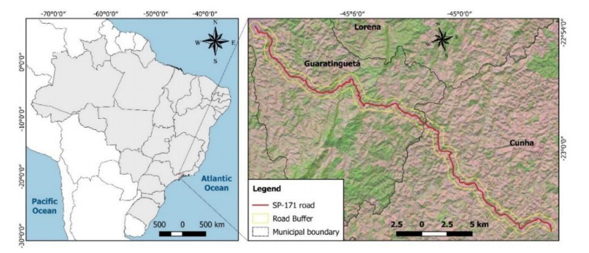
Mass movement susceptibility mapping from rainfall data and in situ site characterization constitute an important approach for preventing geological-geotechnical accidents on railroads and highways. A comprehensive site characterization program was conducted to identify slopes with mass movements along the 44 km of SP-171 road in the state of Sã o Paulo, Brazil. Ninety-two slopes with some degree of instability were found along this section of the road, including rupture scars, active erosive processes and the presence of unstable rock blocks. Two scenarios for mass movement susceptibility (100 mm and 500 mm of accumulated rainfall) were defined by overlaying thematic maps of relief, soil type, geology, accumulated rainfall and declivity using geographic information system-based techniques. The results for both scenarios identified the regions with high and medium susceptibility to mass movements; for the scenario of 100 mm of accumulated rainfall; we found that 27% and 73% of the land area of SP-171 is respectively highly and moderately susceptible to landslide events. For the scenario of 500 mm, we found 58% and 40% to be highly and moderately susceptible areas. This study also allowed us to identify the main geotechnical problems along the 44 km of this road, and thus can be used to guide actions and decisions to avoid or minimize such problems.
Citation: Leila Maria Ramos, Thiago Bazzan, Mariana Ferreira Benessiuti Motta, George de Paula Bernardes, Heraldo Luiz Giacheti. Landslide susceptibility mapping based on rainfall scenarios: a case study from Sao Paulo in Brazil[J]. AIMS Geosciences, 2022, 8(3): 438-451. doi: 10.3934/geosci.2022024
| [1] | Kamsing Nonlaopon, Muhammad Uzair Awan, Sadia Talib, Hüseyin Budak . Parametric generalized (p,q)-integral inequalities and applications. AIMS Mathematics, 2022, 7(7): 12437-12457. doi: 10.3934/math.2022690 |
| [2] | Syed Ghoos Ali Shah, Shahbaz Khan, Saqib Hussain, Maslina Darus . q-Noor integral operator associated with starlike functions and q-conic domains. AIMS Mathematics, 2022, 7(6): 10842-10859. doi: 10.3934/math.2022606 |
| [3] | Aisha M. Alqahtani, Rashid Murtaza, Saba Akmal, Adnan, Ilyas Khan . Generalized q-convex functions characterized by q-calculus. AIMS Mathematics, 2023, 8(4): 9385-9399. doi: 10.3934/math.2023472 |
| [4] | Shuhai Li, Lina Ma, Huo Tang . Meromorphic harmonic univalent functions related with generalized (p, q)-post quantum calculus operators. AIMS Mathematics, 2021, 6(1): 223-234. doi: 10.3934/math.2021015 |
| [5] | Xhevat Z. Krasniqi . Approximation of functions in a certain Banach space by some generalized singular integrals. AIMS Mathematics, 2024, 9(2): 3386-3398. doi: 10.3934/math.2024166 |
| [6] | Bo Wang, Rekha Srivastava, Jin-Lin Liu . Certain properties of multivalent analytic functions defined by q-difference operator involving the Janowski function. AIMS Mathematics, 2021, 6(8): 8497-8508. doi: 10.3934/math.2021493 |
| [7] | Maimoona Karim, Aliya Fahmi, Shahid Qaisar, Zafar Ullah, Ather Qayyum . New developments in fractional integral inequalities via convexity with applications. AIMS Mathematics, 2023, 8(7): 15950-15968. doi: 10.3934/math.2023814 |
| [8] | Li Xu, Lu Chen, Ti-Ren Huang . Monotonicity, convexity and inequalities involving zero-balanced Gaussian hypergeometric function. AIMS Mathematics, 2022, 7(7): 12471-12482. doi: 10.3934/math.2022692 |
| [9] | Ebrahim Amini, Mojtaba Fardi, Shrideh Al-Omari, Rania Saadeh . Certain differential subordination results for univalent functions associated with q-Salagean operators. AIMS Mathematics, 2023, 8(7): 15892-15906. doi: 10.3934/math.2023811 |
| [10] | Ye-Cong Han, Chuan-Yu Cai, Ti-Ren Huang . Monotonicity, convexity properties and inequalities involving Gaussian hypergeometric functions with applications. AIMS Mathematics, 2022, 7(4): 4974-4991. doi: 10.3934/math.2022277 |
Mass movement susceptibility mapping from rainfall data and in situ site characterization constitute an important approach for preventing geological-geotechnical accidents on railroads and highways. A comprehensive site characterization program was conducted to identify slopes with mass movements along the 44 km of SP-171 road in the state of Sã o Paulo, Brazil. Ninety-two slopes with some degree of instability were found along this section of the road, including rupture scars, active erosive processes and the presence of unstable rock blocks. Two scenarios for mass movement susceptibility (100 mm and 500 mm of accumulated rainfall) were defined by overlaying thematic maps of relief, soil type, geology, accumulated rainfall and declivity using geographic information system-based techniques. The results for both scenarios identified the regions with high and medium susceptibility to mass movements; for the scenario of 100 mm of accumulated rainfall; we found that 27% and 73% of the land area of SP-171 is respectively highly and moderately susceptible to landslide events. For the scenario of 500 mm, we found 58% and 40% to be highly and moderately susceptible areas. This study also allowed us to identify the main geotechnical problems along the 44 km of this road, and thus can be used to guide actions and decisions to avoid or minimize such problems.
In this paper, we primarily focus on investigating different properties of generalized (p,q)-elliptic integrals and the generalized (p,q)-Hersch-Pfluger distortion function. In recent years, mathematicians have made significant progress in studying inequalities and various properties related to complete elliptic integrals, especially Legendre elliptic integrals and generalized complete elliptic integrals of the first and second types [3,4,5,10,11,23,26].
We first introduce some necessary notation. For complex numbers a,b,c with c≠0,−1,−2,…, and x∈(−1,1), the Gaussian hypergeometric function [9] is defined as follows:
| F(a,b;c;x)=2F1(a,b;c;x)=∞∑n=0(a,n)(b,n)(c,n)xnn!, | (1.1) |
where (a,n)≡a(a+1)⋯(a+n−1) is the shifted factorial function for n∈N+, and (a,0)=1 for a≠0. As we all know, 2F1(a,b;c;x) has many important applications in the theory of geometric functions and several other contexts [19]. Many special functions in mathematical physics are special or limit cases of this function [1]. Bhayo studied a new form of the generalized (p,q)-complete elliptic integrals as an application of generalized (p,q)-trigonometric functions [6]. In recent years, the generalization of classical trigonometric functions has attracted significant interest [8,20]. For this, we need the generalized arcsine function arcsinp,q(x) and the generalized πp,q. For p,q∈(1,∞), set
| arcsinp,q(x)≡∫x0dt(1−tq)1/p,x∈[0,1], |
and the generalized πp,q is the number defined by
| πp,q=2arcsinp,q(1)≡2∫10dt(1−tq)1/p=2qB(1−1p,1q), |
where B is the beta function. For Rex>0 and Rey>0, the classical gamma function Γ(x) and beta function B(x,y) are respectively defined as
| Γ(x)=∫∞0e−ttx−1dt,B(x,y)=Γ(x)Γ(y)Γ(x+y). |
Clearly, arcsinp,q(x) is an increasing homeomorphism from [0,1] onto [0,πp,q/2], and its inverse function is the generalized (p,q)-sine function sinp,q is defined on the interval [0,πp,q/2]. Moreover, the function sinp,q can be extended to the interval [0,πp,q] by
| sinp,q(x)=sinp,q(πp,q−x),x∈[πp,q/2,π]. |
sinp,q can be also extended to the whole R, and the generalized (p,q)-sine function reduces to the classical sine function for p=q=2.
Applying the definitions of sinp,q(x) and πp,q, we can define the generalized (p,q)-elliptic integrals of the first kind Kp,q and of the second kind Ep,q by
| Kp,q(r)=∫πp,q/20dt(1−rqsinqp,q(t))1−1/p=∫10dt(1−tq)1/p(1−rqtq)1−1/p |
and
| Ep,q(r)=∫πp,q/20(1−rqsinqp,q(t))1/pdt=∫10(1−rqtq1−tq)1/pdt |
respectively, for p,q∈(1,∞), r∈(0,1).
As a special case of the Gaussian hypergeometric function, these generalized (p,q)-elliptic integrals can be represented by Gaussian hypergeometric functions [15] as
| {Kp,q=Kp,q(r)=πp,q22F1(1−1p,1q;1−1p+1q;rq)K′p,q=K′p,q(r)=Kp,q(r′)Kp,q(0)=πp,q2,Kp,q(1)=∞ | (1.2) |
and
| {Ep,q=Ep,q(r)=πp,q22F1(−1p,1q;1−1p+1q;rq)E′p,q=E′p,q(r)=Ep,q(r′)Ep,q(0)=πp,q2,Ep,q(1)=1, | (1.3) |
where p,q∈(1,∞), r∈(0,1), r′=(1−rq)1/q. If p=q=2, we can derive the classical complete elliptic integrals K and E, which are well-known complete elliptic integrals of the first kind and second kind, respectively. These complete elliptic integrals play an important role in many branches of quasiconformal mapping, complex analysis, and physics.
In 2017, Yang et al. [24] showed that the ratio K(r)/ln(c/r′) is strictly concave if and only if c=e4/3 on (0,1), and K(r)/ln(1+4/r′) is strictly convex on (0,1).
In 2019, Wang et al. [22] presented the convexity of the function (E′a−r2K′a)/r′2 and some properties of the function αKa(rα) with respect to the parameter α.
In 2020, Huang et al. [13] established monotonicity properties for certain functions involving the complete p-elliptic integrals of the first and second kinds. They also presented the inequality π/2−log2+log(1+1/r′)+α(1−r′)<Kp(r)<π/2−log2+log(1+1/r′)+β(1−r′) which holds for all r∈(0,1) with the best possible constants α and β. Moreover, these generalized elliptic integrals have significant applications in the theory of geometric functions and in the theory of mean values. More properties and applications of these integrals are given in [7,13,17,21,22,24,25].
The generalized (p,q)-elliptic integrals of the first kind Kp,q and of the second kind Ep,q satisfy the following Legendre relation:
| Kp,q(r)E′p,q(r)+K′p,q(r)Ep,q(r)−Kp,q(r)K′p,q(r)=πp,q2. | (1.4) |
This relation has important applications in many areas of mathematics and physics, including celestial mechanics, quantum mechanics, and statistical mechanics. when p=q=2, the equation reduces to the classical Legendre relation.
Inspired by the papers [22], [24] and [13], we can consider extending the results of K(r), Ka(r) and Kp(r) to the generalized (p,q)-elliptic integrals of the first kind Kp,q.
A generalized (p,q)-modular equation of degree h>0 is
| 2F1(a,b;c;1−sq)2F1(a,b;c;sq)=h2F1(a,b;c;1−rq)2F1(a,b;c;rq),r∈(0,1), | (1.5) |
which a,b,c>0 with a+b≥c. Using the decreasing homeomorphism μp,q:(0,1)→(0,∞) defined by
| μp,q(r)=πp,q2K′p,q(r)Kp,q(r), |
for p,q∈(1,∞). The function μp,q is called the generalized (p,q)-Gr¨otzsch ring function, we can rewrite (1.5) as
| μp,q(s)=hμp,q(r),r∈(0,1). | (1.6) |
The solution of (1.6) is given by
| s=φp,qK(r)=μ−1p,q(μp,q(r)/K). | (1.7) |
For p,q∈(1,∞), r∈(0,1), K∈(0,∞), we have
| φp,qK(r)q+φp,q1/K(r′)q=1. | (1.8) |
The function φp,qK(r) is referred to as the generalized (p,q)-Hersch-Pfluger distortion function with degree K=1/h. For p=q=2, the functions μp,q(r) and φp,qK(r) reduces to well-known special cases that Gr¨otzsch ring function μ(r) and Hersch-Pfluger distortion function φK(r), respectively, which play important role in the theory of plane quasiconformal mappings.
In 2015, Alzer et al. [2] studied the monotonicity, convexity, and concavity properties of the function μ(rα)/α, and established various Gr¨otzsch ring functional inequalities based on these properties.
In [3], the authors focused on studying the properties of the generalized Gr¨otzsch ring function μa(r) and the generalized Hersch-Pfluger distortion function φaK(r). They derived various inequalities involving μa(r) and r−1/KφaK(r) by utilizing the monotonicity, concavity, and convexity of the functions μa(r), r−1/KφaK(r), log(1/φaK(e−x)), and φaK(rx)/φaK(x).
In 2022, Lin et al. [16] explored the monotonicity and convexity properties of the function μp,q(r) and obtained sharp functional inequalities that sharpen and extend some existing results on the modulus of μ(r).
Inspired by the papers [3], [12], and [16], our motivation is to extend the existing results of the functions φK(r) and φaK(r) to the generalized (p,q)-Hersch-Pfluger distortion function. Our goal is to gain the properties of the generalized (p,q)-Hersch-Pfluger distortion function and derive sharp functional inequalities for this function.
Our main objective of this paper is to investigate various properties of the generalized (p,q)-elliptic integrals and the generalized (p,q)-Hersch-Pfluger distortion function. We specifically focus on establishing complete monotonicity, logarithmic, geometric concavity, and convexity properties of certain functions involving these generalized integrals and arcsine functions. Additionally, they derive several sharp functional inequalities for the generalized (p,q)-Hersch-Pfluger distortion function, which improve upon and generalize existing results. Apart from the introduction, this paper consists of three additional sections. Section 2 contains some preliminaries as well as several formulas and lemmas. In Section 3, we present some of the major results regarding the generalized (p, q)-elliptic integrals and provide their proof. In Section 4, we study the generalized (p, q)-Hersch-Pfluger distortion function, and present some of the major results and provide their proof.
In this section, we present several formulas and lemmas that have been extensively utilized in the paper. These formulas and lemmas play a crucial role in the analysis and proofs of the major results. Throughout this paper, we denote p,q∈(1,∞), r∈(0,1) and r′=(1−rq)1/q.
Lemma 2.1. [16] Derivative formulas:
| (1)dKp,qdr=Ep,q−r′qKp,qrr′q,(2)dEp,qdr=q(Ep,q−Kp,q)pr,(3)dμp,q(r)dr=−π2p,q4rr′qK2p,q,(4)d(Ep,q−r′qKp,q)dr=(p−q)(Kp,q−Ep,q)+p(q−1)rqKp,qpr,(5)d(Kp,q−Ep,q)dr=(p−qr′q)Ep,q+(q−p)r′qKp,qprr′q. |
Based on the derivative formula Lemma 2.1, we derive the derivative formulas of the function φp,qK(r) in the following lemma.
Lemma 2.2. Let p,q∈(1,∞), then
| ∂φp,qK(r)∂r=ss′qKp,q(s)K′p,q(s)rr′qKp,q(r)K′p,q(r)=1Kss′qKp,q(s)2rr′qKp,q(r)2=Kss′qK′p,q(s)2rr′qK′p,q(r)2 |
for r∈(0,1).
Proof. By the definitions of s=φp,qK(r), μp,q(s)=μp,q(r)/K, and the derivative formulas of Kp,q(r), we can derive the following equation
| −π2p,q4ss′qKp,q(s)2⋅∂s∂r=−1Kπ2p,q4rr′qKp,q(r)2, |
then the derivative formulas of φp,qK(r) is following.
Lemma 2.3. [4] For p∈[0,∞), let I=[0,p), and suppose that f,g:I→[0,∞) are functions such that f(x)/g(x) is decreasing on I∖{0} and g(0)=0, g(x)>0 for x>0. Then
| f(x+y)(g(x)+g(y))≤g(x+y)(f(x)+f(y)), |
for x,y,x+y∈I. Moreover, if the monotoneity of f(x)/g(x) is strict, then the above inequality is also strict on I∖{0}.
The following result is a monotone form of L'Hˆopital's Rule [4] and will be useful in deriving monotoneity properties and obtaining inequalities.
Lemma 2.4. [4] For −∞<a<b<∞, let f,g:[a,b]→R be continuous on [a,b], and be differentiable on (a,b). Let g′(x)≠0 on (a,b). If f′(x)/g′(x) is increasing (decreasing) on (a,b), then so are
| [f(x)−f(a)]/[g(x)−g(a)]and[f(x)−f(b)]/[g(x)−g(b)]. |
If f′(x)/g′(x) is strictly monotone, then the monotonicity in the conclusion is also strict.
The following lemma presents some known results of generalized (p,q)-elliptic integrals, which can be utilized to prove the main results of this paper.
Lemma 2.5. [14] For p,q∈(1,∞), r∈(0,1), a=1−1/p,b=a+1/q, then the functions
(1) h1(r)=Ep,q(r)−r′qKp,q(r)rq is strictly increasing and convex from (0,1) onto (aπp,q/(2b),1).
(2) h2(r)=Ep,q(r)−r′qKp,q(r)rqKp,q(r) is strictly decreasing from (0,1) onto (0,a/b).
(3) h3(r)=r′cKp,q(r) is decreasing(increasing) on (0,1) iff c≥a/b (c≤0 respectively) with h3((0,1))=(0,πp,q/2) if c≥a/b.
(4) h4(r)=Kp,q(r)−Ep,q(r)rqKp,q(r) is increasing from (0,1) onto (1/(qb),1).
(5) h5(r)=r′qKp,q(r)/Ep,q(r) is strictly decreasing from (0,1) onto itself.
Lemma 2.6. For r∈(0,1), K,p,q∈(1,∞), let s=φp,qK(r),t=φp,q1/K(r).
(1) The function f(r)=Kp,q(s)/Kp,q(r) is increasing from (0,1) onto (1,K).
(2) For q>3p−4p−1, the function g(r)=s′q/2Kp,q(s)2r′q/2Kp,q(r)2 is decreasing from (0,1) onto (0,1).
Proof. (1) According to the Lemma 2.1, we have
| K2p,q(r)f′(r)=Kp,q(s)rr′qK′p,q(r){K′p,q(s)[Ep,q(s)−s′qKp,q(s)]−K′p,q(r)[Ep,q(r)−r′qKp,q(r)]}. |
Denote
| f1(r)=K′p,q(r)[Ep,q(r)−r′qKp,q(r)]=rqK′p,q(r)[Ep,q(r)−r′qKp,q(r)rq]. |
By applying Lemma 2.5(1)(3) and considering s>r, we can conclude that f1(r) is increasing. Hence, we can determine that f′(r) is positive. Therefore, we can deduce that f(r) is an increasing function. For the limiting values, we have limr→0+f(r)=1 and limr→1−f(r)=K.
(2) Let
| g1(r)=K′p,q(r)[qrqKp,q(r)−4(Ep,q(r)−r′qKp,q(r))]=rqK′p,q(r)Kp,q(r)[q−4Ep,q(r)−r′qKp,q(r)rqKp,q(r)]. |
By differentiation, we have
| [r′q/2Kp,q(r)2]2g′(r)=−s′q/2Kp,q(s)2Kp,q(r)2rr′q/2K′p,q(r)(g1(s)−g1(r)). |
If q>3p−4p−1, g1(r) is increasing by Lemma 2.5(2) and (3), thus g′(r) is negative for s>r. Hence g(r) is decreasing, the limiting values follow from the definitions (1.2) and (1.7)
| limr→0+g(r)=1,limr→1−g(r)=0. |
Lemma 2.7. For r∈(0,1) and p,q∈(1,∞), the inequality
| rqKp,q(r)2N(r)>1q |
holds.
Proof. Let M(r)=rqKp,q(r)2/N(r), M1(r)=N(r)/(rqKp,q(r)), we have
| M1(r)=1rqKp,q(r){qpKp,q(r)(Ep,q(r)−r′qKp,q(r))+Ep,q(r)(Kp,q(r)−Ep,q(r))−(qp−q+1)rqKp,q(r)Ep,q(r)}=qpEp,q(r)−r′qKp,q(r)rq+Ep,q(r)Kp,q(r)−Ep,q(r)rqKp,q(r)−(qp−q+1)Ep,q(r). |
According to Lemma 2.5, we have
| M1(r)<qp+q(1−1p)Ep,q(r)<qπp,q2≤qKp,q(r), |
and
| M(r)=Kp,q(r)/M1(r)>1/q. |
Lemma 2.8. For r∈(0,1), p,q∈(1,∞), the function
| h(r)=1log(1/r)−Ep,q(r)−r′qKp,q(r)r′qKp,q(r) |
is strictly increasing from (0,1) onto (0,∞).
Proof. By differentiation, we have
| h′(r)=1r(log(1/r))2−N(r)r(r′qKp,q(r))2=N(r)rq+1(log(1/r))2Kp,q(r)2[rqKp,q(r)2N(r)−(rq/2r′qlog(1r))2], |
where N(r)=qpKp,q(r)(Ep,q(r)−r′qKp,q(r))+Ep,q(r)(Kp,q(r)−Ep,q(r))−(qp−q+1)rqKp,q(r)Ep,q(r).
Let h2(r)=rq/2log(1/r), h3(r)=r′q, then h1(r)=h2(r)/h3(r), and h2(1−)=h3(1−)=0.
| h′2(r)h′3(r)=−1qrq/2[q2log(1/r)−1]. |
By Lemma 2.4, the function h1(r) is strictly increasing from (0,1) onto (0,1/q). According to Lemma 2.7, we conclude that rqKp,q(r)2/N(r)>1/q. Therefore, it is easy to check that h(r) is increasing. For the limiting values, limr→0+h(r)=0. Since
| limr→1−r′qKp,q(r)=0,limr→1−r′qlog(1/r)=q,limr→1−Kp,q(r)=∞, |
we have
| limr→1−h(r)=limr→1−1r′qKp,q(r){r′qKp,q(r)log(1/r)−(Ep,q(r)−r′qKp,q(r))}=∞. |
In this section, we present some of the main results regarding the generalized (p,q)-elliptic integrals.
Theorem 3.1. For p,q∈(1,∞), the function Fp,q(r)=(E′p,q(r)−rqK′p,q(r))/r′q is concave on (0,r∗0) and convex on (r∗0,1) for some point r∗0∈(0,1).
Proof. Let F(r)=(Ep,q(r)−r′qKp,q(r))/rq, by the definitions (1.2) and (1.3), which can be expressed as
| F(r)=Ep,q(r)−r′qKp,q(r)rq=πp,q2rq[F(−1p,1q;1−1p+1q;rq)−r′qF(1−1p,1q;1−1p+1q;rq)]=πp,q2rq[∞∑n=0((−1p,n)(1q,n)(1−1p+1q,n)n!−(1−1p,n)(1q,n)(1−1p+1q,n)n!)rqn+∞∑n=0(1−1p,n)(1q,n)(1−1p+1q,n)n!rq(n+1)]=πp,q2∞∑n=0(1−1p,n)(1q,n)(1−1p+1q,n+1)(n+1)!(1−1p)(n+1)rqn=aπp,q2(a+b)2F1(a,b;a+b+1;rq), |
with a=1−1/p,b=1/q. This implies that
| Fp,q(r)=E′p,q(r)−rqK′p,q(r)r′q=aπp,q2(a+b)2F1(a,b;a+b+1;r′q). |
By differentiation, we have
| F′p,q(r)=−a2bqπp,q2(a+b)(a+b+1)rq−12F1(a+1,b+1;a+b+2;r′q). |
Hence,
| −2(a+b)(a+b+1)a2bqπp,qF″p,q(r)=(q−1)rq−22F1(a+1,b+1;a+b+2;r′q)−q(a+1)(b+1)a+b+2r2q−22F1(a+2,b+2;a+b+3;r′q). |
According to [4, Theorem 1.19(10)],
| 2F1(a,b;c;x)=(1−x)c−a−b2F1(c−a,c−b;c;x)(a+b>c,a,b,c>0), |
we have
| −2(a+b)(a+b+1)a2bqπp,qF″p,q(r)=(q−1)rq−22F1(a+1,b+1;a+b+2;r′q)−q(a+1)(b+1)a+b+2rq−22F1(a+1,b+1;a+b+3;r′q)=(q−1)rq−22F1(a+1,b+1;a+b+3;r′q)[2F1(a+1,b+1;a+b+2;r′q)2F1(a+1,b+1;a+b+3;r′q)−qq−1(a+1)(b+1)a+b+2]. | (3.1) |
Let
| F1(x)=2F1(a+1,b+1;a+b+2;x)2F1(a+1,b+1;a+b+3;x)=∑∞n=0anxn∑∞n=0bnxn, |
it is easy to obtain that F1(x) is strictly increasing from (0,1) onto (1,∞), since
| anbn=a+b+2+na+b+2>1. |
Similarly, we can deduce that
| r↦2F1(a+1,b+1;a+b+2;r′q)2F1(a+1,b+1;a+b+3;r′q)−qq−1(a+1)(b+1)a+b+2 |
is strictly decreasing from (0,1) onto (1−b(2a+b+2)(1−b)(a+b+2),∞). Therefore, the sign of F″p,q(r) changes from negative to positive on (0,1) by (3.1), we know that there exists r∗0∈(0,1) such that Fp,q(r) is concave on (0,r∗0) and convex on (r∗0,1).
Theorem 3.2. For p,q∈(1,∞), r∈(0,1), α>0, Let Hp,q(α)=αKp,q(rα), Gp,q(α)=Kp,q(rα)/α. Then
(1) The function α↦Hp,q(α) is strictly increasing and log-concave on (0,∞);
(2) The function α↦1/Hp,q(α) is strictly convex on (0,∞);
(3) The function α↦Gp,q(α) is strictly decreasing and log-convex on (0,∞).
Proof. (1) Let t=rα, then dt/dα=tlogr<0, and
| dHp,q(α)dα=Kp,q(t)+αEp,q(t)−t′qKp,q(t)t′qlogr=Kp,q(t)−Ep,q(t)−t′qKp,q(t)t′qlog(1t)=Kp,q(t)log(1t)[1log(1/t)−Ep,q(t)−t′qKp,q(t)t′qKp,q(t)]. |
Hence, the monotonicity of Hp,q(α) follows from Lemma 2.8.
By logarithmic differentiation,
| d(logHp,q(α))dα=1α−Ep,q(t)−t′qKp,q(t)t′qKp,q(t)log(1r)=log(1r)[1log(1/t)−Ep,q(t)−t′qKp,q(t)t′qKp,q(t)]. |
It is not difficult to verify that d(logHp,q(α))/dα is strictly increasing with respect to t by Lemma 2.8, and is strictly decreasing with respect to α. Thus the function α↦Hp,q(α) is strictly increasing and log-concave on (0,∞).
(2) Since t=rα, then α=log(1/t)/log(1/r). Differentiating 1/Hp,q(α) yields
| ddα(1Hp,q(α))=−1Hp,q(α)2Kp,q(t)log(1t)[1log(1/t)−Ep,q(t)−t′qKp,q(t)t′qKp,q(t)]=−1α2Kp,q(t)2Kp,q(t)log(1t)h(t)=−(log1r)2h(t)log(1/t)Kp,q(t), | (3.2) |
where h(t) is defined in Lemma 2.8. Let f(r)=log(1/r)Kp,q(r), f1(r)=log(1/r), f2(r)=1/Kp,q(r), We clearly see that f1(1)=f2(1)=0, then
| f′1(r)f′2(r)=r′qKp,q(r)2Ep,q(r)−r′qKp,q(r)=rqEp,q(r)−r′qKp,q(r)⋅r′qKp,q(r)2rq, |
which is decreasing follows from Lemma 2.5(1), (3). Hence the function f(r) is decreasing from (0,1) onto (0,∞) by Lemma 2.4. Therefore, it follows from Lemma 2.8 and (3.2) that the function α↦1/Hp,q(α) is strictly convex on (0,∞).
(3) Since t=rα, and dt/dα=tlogr<0, simple computations yields
| dGp,q(α)dα=1α[Ep,q(t)−t′qKp,q(t)t′qlogr−Kp,q(t)α]=1α[Ep,q(t)−t′qKp,q(t)t′qlogr−Kp,q(t)logrlogt]=Kp,q(t)logrα[Ep,q(t)−t′qKp,q(t)t′qKp,q(t)+1log(1/t)]. |
Let g(r)=Ep,q(r)−r′qKp,q(r)r′qKp,q(r)+1log(1/r), we have
| g′(r)=N(r)rq+1(log(1/r))2Kp,q(r)2[rqKp,q(r)2N(r)+(rq/2r′qlog(1r))2], |
is positive by Lemma 2.8, where the defition of N(r) is in Lemma 2.8. Hence the function g(r) is increasing from (0,1) onto (0,∞). Since logr<0, the monotonicity of the function Gp,q(α) follows immediately.
Since logGp,q(α)=logKp,q(t)−logα, by differentiation, we obtain that
| d(logGp,q(α))dα=Ep,q(t)−t′qKp,q(t)t′qKp,q(t)logr−1α=Ep,q(t)−t′qKp,q(t)t′qKp,q(t)logr−logrlogt=logr[Ep,q(t)t′qKp,q(t)−1+1log(1/t)]. | (3.3) |
It follows from (3.3) and Lemma 2.5(5) that d(logGp,q(α))/dα is strictly decreasing with respect to t. Therefore, Gp,q(α) is log-convex on (0,∞) with respect to α.
Next, we apply Theorem 3.2 to obtain the inequality involving the generalized (p,q)-elliptic integrals Kp,q.
Corollary 3.1. For p,q∈(1,∞).
(1) Let α,β be positive numbers with α>β>0. The double inequality
| 1<Kp,q(rβ)Kp,q(rα)<αβ |
holds for all r∈(0,1).
(2) Inequality
| Kp,q(√xy)≥2√log(1/x)log(1/y)log[1/(xy)]√Kp,q(x)√Kp,q(y) |
holds with equality if and only if x=y for all x,y∈(0,1).
(3) Inequality
| 4log[1/(xy)]Kp,q(√xy)≤1log(1/x)Kp,q(x)+1log(1/y)Kp,q(y) |
holds with equality if and only if x=y for all x,y∈(0,1).
(4) Let α,β be positive numbers with α>β>0. The double inequality
| βα<Kp,q(rβ)Kp,q(rα) |
holds for all r∈(0,1).
(5) Inequality
| Kp,q(√xy)≤12log(1xy)√Kp,q(x)Kp,q(y)log(1/x)log(1/y) |
holds with equality if and only if x=y for all x,y∈(0,1).
Proof. (1) By utilizing the monotonicity of the function Hp,q(α) stated in Theorem 3.2, along with the monotonicity of the function Kp,q(r), we can establish that αKp,q(rα)>βKp,q(rβ). Consequently, the double inequality holds.
(2) Since the function α↦Hp,q(α) is strictly log-concave on (0,∞), we can deduce that
| logHp,q(α+β2)≥12(logHp,q(α)+logHp,q(β))⇒Hp,q(α+β2)≥√Hp,q(α)Hp,q(β) |
with equality if and only if α=β for α,β>0. For x,y∈(0,1) and set
| α=log(1/x)log(1/r),β=log(1/y)log(1/r). |
Simple computations yields
| Hp,q(α)=αKp,q(rα)=log(1/x)log(1/r)Kp,q(x),Hp,q(β)=βKp,q(rβ)=log(1/y)log(1/r)Kp,q(y), | (3.4) |
| Hp,q(α+β2)=12log[1/(xy)]log(1/r)Kp,q(√xy). | (3.5) |
Hence, the inequality
| Kp,q(√xy)≥2√log(1/x)log(1/y)log[1/(xy)]√Kp,q(x)√Kp,q(y) |
hold with equality if and only if x=y.
(3) Since the function α↦1/Hp,q(α) is strictly convex on (0,∞), we get
| 1Hp,q(α+β2)≤12(1Hp,q(α)+1Hp,q(β)) | (3.6) |
with equality if and only if α=β for α,β>0. Set
| α=log(1/x)log(1/r),β=log(1/y)log(1/r). |
From (3.4)–(3.6), we conclude that the inequality hold with equality if and only if x=y.
(4) Since the function α↦Gp,q(α) is strictly decreasing, and the monotonicity of the function Kp,q(r), we have
| Kp,q(rα)α<Kp,q(rβ)β. |
(5) Since the function α↦Gp,q(α) is log-convex on (0,∞),
| logGp,q(α+β2)≤12(logGp,q(α)+logGp,q(β))⇒Gp,q(α+β2)≤√Gp,q(α)Gp,q(β) |
with equality if and only if α=β for α,β>0. Set
| α=log(1/x)log(1/r),β=log(1/y)log(1/r). |
Simple computations yields
| Gp,q(α)=Kp,q(rα)α=log(1/r)log(1/x)Kp,q(x),Gp,q(β)=Kp,q(rβ)β=log(1/r)log(1/y)Kp,q(y), |
| Gp,q(α+β2)=2log(1/r)log[1/(xy)]Kp,q(√xy). |
Hence, the inequality
| Kp,q(√xy)≤12log(1xy)√Kp,q(x)Kp,q(y)log(1/x)log(1/y) |
hold with equality if and only if x=y.
Remark 3.1. In [22], Wang et al. provided the proof for the convexity of the function (E′a−r2K′a)/r′2 and presented certain properties of the functions αKa(rα) and 1/αKa(rα) with respect to the parameter α. It is worth noting that Theorem 3.1 and Theorem 3.2(1), (2) can be reduced to [22, Theorem 1.1, Theorem 1.3] if p=q=1/a.
In this section, we study the complete monotonicity, logarithmic, geometric concavity and convexity of the generalized (p,q)-Hersch-Pfluger distortion function, and present some of the main results about φp,qK.
Theorem 4.1. For K,p,q∈(1,∞), and q>3p−4p−1, let a=1−1/p,b=1/q, f,g be defined on (0,1] by
| f(r)=r−1/Kφp,qK(r),g(r)=r−Kφp,q1/K(r). |
Then f is decreaseing from (0,1] onto [1,ebR(a,b)(1−1/K)), and g is increasing from (0,1] onto (ebR(a,b)(1−K),1].
Proof. Let s=φp,qK(r), then f(r)=sr1/K, we have
| (r1/K)2f′(r)=sKr1/K−1[(s′q/2Kp,q(s)r′q/2Kp,q(r))2−1]. |
Hence,
| f′(r)f(r)=1Kr[(s′q/2Kp,q(s)r′q/2Kp,q(r))2−1]. |
According to Lemma 2.6(2), f′(r) is negative. Combine with f(1−)=1 and by [18, Theorem 2],
| limr→0+log(r−1/Ks)=limr→0+[(μp,q(s)+logs)−1K(μp,q(r)+logr)]=bR(a,b)(1−1K). |
Let t=φp,q1/K(r), thus r=φp,qK(t) and
| g(r)=φp,qK(t)−K⋅t=(t−1/Kφp,qK(t))−K=f(t)−K. |
According to the monotonicity of f(r), g(r) is increasing on (0,1]. The limiting values can also be derived from [18, Theorem 2].
Next, we utilize Theorem 4.1 to derive the inequality concerning the generalized (p,q)-Hersch-Pfluger distortion function φp,qK.
Corollary 4.1. For K,p,q∈(1,∞), and q>3p−4p−1, let a=1−1/p,b=1/q, then
(1) The double inequality
| |φp,qK(r)−φp,qK(s)|≤φp,qK(|r−s|)≤ebR(a,b)(1−1/K)|r−s|1/K | (4.1) |
hold with equality if and only if r=s.
(2) The double inequality
| |φp,q1/K(r)−φp,q1/K(s)|≥φp,q1/K(|r−s|)≥ebR(a,b)(1−K)|r−s|K | (4.2) |
hold with equality if and only if r=s.
Proof. (1) According to Lemma 2.3 and the monotonicity of the function f(r)=r−1/Kφp,qK(r), we can conclude that
| φp,qK(x+y)≤φp,qK(x)+φp,qK(y) |
for x,y∈(0,1). Set r=x+y and s=y, we get
| |φp,qK(r)−φp,qK(s)|≤φp,qK(|r−s|). |
According to f(r) is decreaseing from (0,1] onto [1,ebR(a,b)(1−1/K)), we obtain that
| φp,qK(|r−s|)≤ebR(a,b)(1−1/K)|r−s|1/K |
with equality if and only if r=s.
(2) By Lemma 2.3 and the monotonicity of g(r), we have
| φp,q1/K(x)+φp,q1/K(y)≤φp,q1/K(x+y) |
for x,y∈(0,1). Set r=x+y and s=y, we obtain that
| |φp,q1/K(r)−φp,q1/K(s)|≥φp,q1/K(|r−s|) |
with equality if and only if r=s.
According to g(r) increasing from (0,1] onto (ebR(a,b)(1−K),1], we get
| φp,q1/K(|r−s|)≥ebR(a,b)(1−K)|r−s|K |
with equality if and only if r=s. Therefore, the double inequality (4.2) hold.
Theorem 4.2. For K,p,q∈(1,∞), q>3p−4p−1, the function f(x)=log(1/φp,qK(e−x)) is increasing and convex on (0,∞), g(x)=log(1/φp,q1/K(e−x)) is increasing and concave on (0,∞), and
| φp,qK(r)φp,qK(t)≤(φp,qK(√rt))2,φp,q1/K(r)φp,q1/K(t)≥(φp,q1/K(√rt))2, |
with equality if and only if K=1 for each r,t∈(0,1).
Proof. Let r=e−x,s=φp,qK(r), according to the Lemma 2.6, we have
| f′(x)=1K(s′q/2Kp,q(s)r′q/2Kp,q(r))2 |
is positive and increasing with respect to x. Thus f is increasing and convex. Therefore,
| f(x+y2)≤12(f(x)+f(y)), |
and putting r=e−x,t=e−y, we obtain
| φp,qK(r)φp,qK(t)≤(φp,qK(√rt))2, |
with equality if and only if K=1 for each r,t∈(0,1). The proof for g(x) follows a similar approach.
Theorem 4.3. For K,p,q∈(1,∞), q>3p−4p−1, r∈(0,1), the function f(x)=φp,qK(rx)/φp,qK(x) is increasing from (0,1) onto (r1/K,φp,qK(r)), while function g(x)=φp,q1/K(rx)/φp,q1/K(x) is decreasing from (0,1) onto (φp,q1/K(r),rK). In particular,
| φp,qK(rt)≤φp,qK(r)φp,qK(t),φp,q1/K(rt)≥φp,q1/K(r)φp,q1/K(t), |
with equality if and only if K=1 for each r,t∈(0,1).
Proof. Let t=rx,u=φp,qK(t),s=φp,qK(x),
| f′(x)=uKsx[(u′q/2Kp,q(u)t′q/2Kp,q(t))2−(s′q/2Kp,q(s)x′q/2Kp,q(x))2], |
then
| f′(x)f(x)=1Kx[(u′q/2Kp,q(u)t′q/2Kp,q(t))2−(s′q/2Kp,q(s)x′q/2Kp,q(x))2]. |
Since t<x and s′q/2Kp,q(s)x′q/2Kp,q(x) is decreasing with respect to r by Lemma 2.6, f′(x) is positive on (0,1). For the limiting values, by using L'Hˆopital's Rule, we get
| limr→0+f(r)=r1/K,limr→1−h(r)=φp,qK(r). |
Since the monotonicity of the function f(x), along with the definition of the function φp,qK(r), we obtain
| φp,qK(rt)≤φp,qK(r)φp,qK(t), |
with equality if and only if K=1 for each r,t∈(0,1). The proof for g(x) follows a similar approach. As a result, we will omit the detailed proof.
Theorem 4.4. For K,p∈(1,∞), r∈(0,1), q>3 and p>q(q−3)q2−2q−1, the function f(r) defined by
| f(r)=arcsin(φp,qK(r))arcsin(r1/K) |
is strictly decreasing from (0,1] into [1,e(1−1/K)bR(a,b)), the function g(r) defined by
| g(r)=arcsin(φp,q1/K(r))arcsin(rK) |
is strictly increasing from (0,1] into (e(1−K)bR(a,b),1], where a=1−1/p,b=a+1/q.
Proof. Let s=φp,qK(r), f1(r)=arcsin(s), f2(r)=arcsin(r1/K), f(r)=f1(r)/f2(r). Since f1(0)=f2(0)=0, we have
| f′1(r)f′2(r)=sr1/K(1−r2/K1−r2)1/2s′q−1Kp,q(s)2r′q−1Kp,q(r)2. |
Let f3(r)=s′q−1Kp,q(s)2r′q−1Kp,q(r)2, according to the Lemma 2.1, we have
| [r′q−1Kp,q(r)2]2f′3(r)=−s′q−1Kp,q(s)2Kp,q(r)rr′K′p,q(r)(f4(s)−f4(r)), |
where
| f4(r)=K′p,q(r)[(q−1)rqKp,q(r)−2(Ep,q(r)−r′qKp,q(r))]=rqK′p,q(r)Kp,q(r)[(q−1)−2Ep,q(r)−r′qKp,q(r)rqKp,q(r)]. |
Using Lemma 2.5(2) and (3), we can observe that f4(r) is positive. Consequently, we can deduce that f3(r) is decreasing. As a result, we obtain that f(r) is decreasing on the interval (0,1] by Theorem 4.1. Furthermore, it can be deduced that the monotonicity of g(r) is similar to that of f(r).
Remark 4.1. Theorems 4.1 to 4.4 can be seen as variations and extensions of the results presented in [3, Theorem 1.14, Theorem 1.15, Theorem 6.7, Theorem 6.13]. When p=q=1/a, the results obtained in Theorems 4.1 to 4.4 can be reduced to those obtained in [3].
In this paper, we investigate the properties of the generalized (p,q)-elliptic integrals and the generalized (p,q)-Hersch-Pfluger distortion function. Through our analysis, we have established complete monotonicity, logarithmic, geometric concavity, and convexity properties for certain functions involving these integrals and arcsine functions. These properties provide valuable insights into the behavior of these functions. Furthermore, we have derived several sharp functional inequalities for the generalized (p,q)-elliptic integrals and the generalized (p,q)-Hersch-Pfluger distortion function. These inequalities not only improve upon existing results but also generalize them.
The authors declare that they have not used Artificial Intelligence tools in the creation of this article.
The research was supported by the Natural Science Foundation of China (Grant Nos. 11601485, 11401531).
The authors declare that they have no conflicts of interest.
| [1] |
Ngo PTT, Panahi M, Khosravi K, et al. (2021) Evaluation of deep learning algorithms for national scale landslide susceptibility mapping of Iran. Geosci Front 12: 505–519. https://doi.org/10.1016/j.gsf.2020.06.013 doi: 10.1016/j.gsf.2020.06.013

|
| [2] |
Azarafza M, Ghazifard A, Akgün H, et al. (2018) Landslide susceptibility assessment of South Pars Special Zone, southwest Iran. Environ Earth Sci 77: 1–29. https://doi.org/10.1007/s12665-018-7978-1 doi: 10.1007/s12665-018-7978-1
|
| [3] |
Ayalew L, Yamagishi H (2005) The application of GIS-based logistic regression for landslide susceptibility mapping in the Kakuda-Yahiko Mountains, Central Japan. Geomorphology 65: 15–31. https://doi.org/10.1016/j.geomorph.2004.06.010 doi: 10.1016/j.geomorph.2004.06.010
|
| [4] |
Nanehkaran YA, Mao Y, Azarafza M, et al. (2021) Fuzzy-based multiple decision method for landslide susceptibility and hazard assessment: A case study of Tabriz, Iran. Geomech Eng 24: 407–418. https://doi.org/10.12989/gae.2021.24.5.407 doi: 10.12989/gae.2021.24.5.407
|
| [5] |
Wu Y, Ke Y, Chen Z, et al. (2020) Application of alternating decision tree with AdaBoost and bagging ensembles for landslide susceptibility mapping. Catena 187: 104396. https://doi.org/10.1016/j.catena.2019.104396 doi: 10.1016/j.catena.2019.104396
|
| [6] |
Guo Z, Shi Y, Huang F, et al. (2021) Landslide susceptibility zonation method based on C5.0 decision tree and K-means cluster algorithms to improve the efficiency of risk management. Geoscience Frontiers 12: 101249. https://doi.org/10.1016/j.gsf.2021.101249 doi: 10.1016/j.gsf.2021.101249
|
| [7] | Departamento de Estradas de Rodagem-DER (2017) Parecer técnico—processo nº 000427/07/der/2.017. Engenheiro Hiromiti Nakao CEE/de – projetos, "In press". |
| [8] |
Tajudin N, Ya'acob N, Mohd ali D, et al. (2020) Estimation of TRMM rainfall for landslide occurrences based on rainfall threshold analysis. Int J Electr Comput Eng 10: 3208–3215. https://doi.org/10.11591/ijece.v10i3.pp3208-3215 doi: 10.11591/ijece.v10i3.pp3208-3215
|
| [9] | Pereira JO (1998) Avaliação das condições dos taludes ao longo da rodovia SP - 171 que liga as cidades de Guaratinguetá e Cunha/SP. Relatório das atividades desenvolvidas. UNESP - Guaratinguetá., "In press". |
| [10] | Arrais LS (2000) Estudo geológico e geotécnico dos solos residuais do pré-cambriano da região da rodovia SP-171. Monografia (Graduação em Engenharia Civil). Universidade Estadual Paulista, Guaratinguetá/SP, 2000, "In press". |
| [11] | Instituto Geológico—IG (2010) Relatório de atendimento técnico—PPDC operação 2009/2010. Decreto nº 42585 de 01.12.97 que dispõe sobre o plano preventivo da defesa civil. Available from: https://www.infraestruturameioambiente.sp.gov.br/institutogeologico?s=cunha. |
| [12] | Companhia de Pesquisa de Recursos Minerais—CPRM (2017) Relatório de ação emergencial para delimitação de áreas em alto e muito alto risco a enchentes, inundações e movimentos de massa, Cunha/SP. Available from: https://rigeo.cprm.gov.br/handle/doc/20711. |
| [13] | Instituto de Pesquisas Tecnológicas—IPT (2018) Reavaliação do mapeamento das áreas de risco no município de Cunha/SP. Relatório técnico nº 154.612-205 SDECTI/PATEM Prefeitura Municipal de Cunha. |
| [14] |
Valladares Soares P, Yoshinaga Pereira S, Coelho Simões SJ, et al. (2008) Mapa de infiltração do alto e médio vale do paraíba do sul com base em elementos do meio físico e na precipitação. Revista Ambiente Água 3: 36–42. https://doi.org/10.4136/ambi-agua.40 doi: 10.4136/ambi-agua.40
|
| [15] | Coelho JOM, Zaine JE, Rodrigues FH (2016) Análise fisiográfica, a partir de técnicas de fotointerpretação, aplicada ao mapeamento geológico-geotécnico de obras rodoviárias. Revista Brasileira de Cartografia 68. Available from: http://www.seer.ufu.br/index.php/revistabrasileiracartografia/article/view/44302. |
| [16] | Bazzan T (2018) Análise da suscetibilidade a escorregamentos no município de Guaratinguetá/SP. Monografia (curso de introdução ao geoprocessamento). Instituto Nacional de Pesquisas Espaciais, São José dos Campos. Available from: http://wiki.dpi.inpe.br/lib/exe/fetch.php?media=ser300:trabalho_final_thiago_bazzan.pdf. |
| [17] |
Ribeiro AJA, da Silva CAU, Barroso SHA (2018) Metodologia de baixo custo para mapeamento geotécnico aplicado à pavimentação. Transportes 26: 84–100. https://doi.org/10.14295/transportes.v26i2.1491 doi: 10.14295/transportes.v26i2.1491
|
| [18] | Instituto de Pesquisas Tecnológicas—IPT (2015) Carta de suscetibilidade a movimentos gravitacionais de massa e inundações: município de Guaratinguetá—SP. 1 mapa, color. Escala 1: 50.000. Available from: http://rigeo.cprm.gov.br/xmlui/handle/doc/15176. |
| [19] | Instituto de Pesquisas Tecnológicas—IPT (2015) Carta de suscetibilidade a movimentos gravitacionais de massa e inundações: município de Cunha/SP. 1 mapa, color. Escala 1: 75.000. Available from: http://rigeo.cprm.gov.br/jspui/handle/doc/15169. |
| [20] | Bitar OY (2014) Cartas de suscetibilidade a movimentos gravitacionais de massa e inundações: 1: 25.000 (livro eletrônico): nota técnica explicativa/coordenação Omar Yazbek Bitar. São Paulo: IPT—Instituto de Pesquisas Tecnológicas do Estado de São Paulo; Brasília, DF: CPRM—Serviço Geológico. |
| [21] | Instituto de Pesquisas Tecnológicas—IPT (2010) Parecer técnico, n. 18.745 - 301 - i/122, 2010. |
| [22] | Simões SJC, Bernardes GP, Trannin ICB, et al. (2012) Relação do meio físico com o manejo sustentável de plantio de eucalipto em áreas de terrenos acidentados—a fazenda Santa Edwirges, Vale do Paraíba, sudeste do Brasil. Geosciences 31: 431–445. |
| [23] | Empresa Brasileira de Pesquisa Agropecuária—EMBRAPA (2013) Banco de Dados Climáticos do Brasil. Available from: https://www.cnpm.embrapa.br/projetos/bdclima/index.html. |
| [24] |
Rozante JR, Moreira DS, Gonçalves LGG, et al. (2010) Combining TRMM and surface observations of precipitation: technique and validation over South America. Weather Forecast 25: 885–894. https://doi.org/10.1175/2010WAF2222325.1 doi: 10.1175/2010WAF2222325.1
|
| [25] | Santoro J, Mendes RM, Pressinotti MMN, et al. (2008) Correlação entre chuvas e deslizamentos ocorridos durante a operação do plano preventivo de defesa civil em São Paulo. Simpósio Brasileiro de Cartografia Geotécnica e Geoambiental. Available from: <https://www.researchgate.net/publication/310801390_correlacao_entre_chuvas_e_deslizamentos_ocorridos_durante_a_operacao_do_plano_preventivo_de_defesa_civil_em_sao_paulo_sp/link/5838371308aef00f3bf9e94c/download. |
| [26] | Alaska Satellite Facility—ASF/Distributed active archive centers—DAAC (2020) ALOS PALSAR Hi-Res terrain corrected. Available from: https://search.asf.alaska.edu. |
| [27] | Departamento de Águas e Energia Elétrica—DAEE (1984) Mapa geológico na escala original 1: 250 000. Universidade Estadual Paulista—UNESP. |
| [28] | Oliveira JB, Camargo MN, Rossi M, et al. (1999) Mapa pedológico do estado de São Paulo: legenda expandida escala 1: 500.000. Campinas: Instituto Agronômico/EMBRAPA solos. |
| [29] | Companhia de Pesquisa de Recursos Minerais—CPRM (2020) Cartas de suscetibilidade a movimentos gravitacionais de massa e inundações—São Paulo. Available from: http://www.cprm.gov.br/publique/gestao-territorial/prevencao-de-desastres/cartas-de-suscetibilidade-a-movimentos-gravitacionais-de-massa-e-inundacoes---sao-paulo-5088.html. |
| [30] | Ramos LM, Bernardes GP, Motta MFB, et al. (2019) Retroanálise da ruptura de um talude rodoviário na SP-171: Cunha/SP. Ⅸ Congresso Brasileiro de Geotecnia Ambiental. Ⅷ Congresso Brasileiro de Geossintéticos. São Carlos, São Paulo, Brasil© IGS-Brasil/ABMS. Available from: http://www.abms.com.br/links/bibliotecavirtual/Regeo-Geossinteticos%202019/Anais_Geossinteticos_REGEO2019.pdf. |
| [31] |
Antunes F, Campos T, Polivanov H, et al. (2013) Desenvolvimento de classes e unidades geo-pedológicas a partir da interação entre a pedologia e a geotecnia. Geotecnia, 61–79. https://doi.org/10.14195/2184-8394_127_3 doi: 10.14195/2184-8394_127_3
|
| [32] | Silva VCB, Machado PS (2014) SIG na análise ambiental: susceptibilidade erosiva da bacia hidrográfica do córrego mutuca, Nova Lima—Minas Gerais. Revista de Geografia (UFPE). Available from: https://periodicos.ufpe.br/revistas/revistageografia/article/view/229090. |
| [33] | Prefeitura Municipal de Angra dos Reis/RJ (2010) Prefeitura preparou o formulário AVADAN. Available from: https://www.angra.rj.gov.br/noticia.asp?vid_noticia=30386&indexsigla=imp. |
| [34] | Gerscovich DMS (2016) Estabilidade de taludes. 2 ed., São Paulo: Oficina de textos. |
| [35] |
Di B, Stamatopoulos CA, Stamatopoulos AC, et al. (2021) Proposal, application and partial validation of a simplified expression evaluating the stability of sandy slopes under rainfall conditions. Geomorphology 395: 107966. https://doi.org/10.1016/j.geomorph.2021.107966 doi: 10.1016/j.geomorph.2021.107966
|
| [36] |
Take WA, Bolton MD, Wong PCP, et al. (2004) Evaluation of landslide triggering mechanisms in model fill slopes. Landslides 1: 173–184. https://doi.org/10.1007/s10346-004-0025-1 doi: 10.1007/s10346-004-0025-1
|
| [37] |
Huang Y, Zhao L (2018) Review on landslide susceptibility mapping using support vector machines. Catena 165: 520–529. https://doi.org/10.1016/j.catena.2018.03.003 doi: 10.1016/j.catena.2018.03.003
|
| [38] |
Chen X, Chen W (2021) GIS-based landslide susceptibility assessment using optimized hybrid machine learning methods. Catena 196: 104833. https://doi.org/10.1016/j.catena.2020.104833 doi: 10.1016/j.catena.2020.104833
|
Leila Maria Ramos, Thiago Bazzan, Mariana Ferreira Benessiuti Motta, George de Paula Bernardes, Heraldo Luiz Giacheti. Landslide susceptibility mapping based on rainfall scenarios: a case study from Sao Paulo in Brazil[J]. AIMS Geosciences, 2022, 8(3): 438-451. doi: 10.3934/geosci.2022024


 DownLoad: