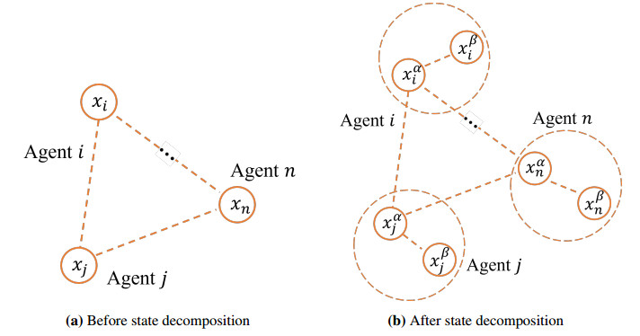
In this paper, we study the privacy-preserving distributed optimization problem on directed graphs, aiming to minimize the sum of all agents' cost functions and protect the sensitive information. In the distributed optimization problem of directed graphs, agents need to exchange information with their neighbors to obtain the optimal solution, and this situation may lead to the leakage of privacy information. By using the state decomposition method, the algorithm ensures that the sensitive information of the agent will not be obtained by attackers. Before each iteration, each agent decomposes their initial state into two sub-states, one sub-state for normal information exchange with other agents, and the other sub-state is only known to itself and invisible to the outside world. Unlike traditional optimization algorithms applied to directed graphs, instead of using the push-sum algorithm, we introduce the external input, which can reduce the number of communications between agents and save communication resources. We prove that in this case, the algorithm can converge to the optimal solution of the distributed optimization problem. Finally, a numerical simulation is conducted to illustrate the effectiveness of the proposed method.
Citation: Mengjie Xu, Nuerken Saireke, Jimin Wang. Privacy-preserving distributed optimization algorithm for directed networks via state decomposition and external input[J]. Electronic Research Archive, 2025, 33(3): 1429-1445. doi: 10.3934/era.2025067
In this paper, we study the privacy-preserving distributed optimization problem on directed graphs, aiming to minimize the sum of all agents' cost functions and protect the sensitive information. In the distributed optimization problem of directed graphs, agents need to exchange information with their neighbors to obtain the optimal solution, and this situation may lead to the leakage of privacy information. By using the state decomposition method, the algorithm ensures that the sensitive information of the agent will not be obtained by attackers. Before each iteration, each agent decomposes their initial state into two sub-states, one sub-state for normal information exchange with other agents, and the other sub-state is only known to itself and invisible to the outside world. Unlike traditional optimization algorithms applied to directed graphs, instead of using the push-sum algorithm, we introduce the external input, which can reduce the number of communications between agents and save communication resources. We prove that in this case, the algorithm can converge to the optimal solution of the distributed optimization problem. Finally, a numerical simulation is conducted to illustrate the effectiveness of the proposed method.

| [1] |
A. Priolo, A. Gasparri, E. Montijano, C. Sagues, A distributed algorithm for average consensus on strongly connected weighted digraphs, Automatica, 50 (2014), 946–951. https://doi.org/10.1016/j.automatica.2013.12.026 doi: 10.1016/j.automatica.2013.12.026

|
| [2] |
B. Houska, J. Frasch, M. Diehl, An augmented Lagrangian based algorithm for distributed nonconvex optimization, SIAM J. Optim., 26 (2016), 1101–1127. https://doi.org/10.1137/140975991 doi: 10.1137/140975991
|
| [3] |
R. Mohebifard, A. Hajbabaie, Distributed optimization and coordination algorithms for dynamic traffic metering in urban street networks, IEEE Trans. Intell. Transp. Syst., 20 (2019), 1930–1941. https://doi.org/10.1109/TITS.2018.2848246 doi: 10.1109/TITS.2018.2848246
|
| [4] |
G. Chen, Q. Yang, Distributed constrained optimization for multiagent networks with nonsmooth objective functions, Syst. Control Lett., 124 (2019), 60–67. https://doi.org/10.1016/j.sysconle.2018.12.005 doi: 10.1016/j.sysconle.2018.12.005
|
| [5] |
M. Tajalli, A. Hajbabaie, Distributed optimization and coordination algorithms for dynamic speed optimization of connected and autonomous vehicles in urban street networks, Transp. Res. Part C Emerging Technol., 95 (2018), 497–515. https://doi.org/10.1016/j.trc.2018.07.012 doi: 10.1016/j.trc.2018.07.012
|
| [6] |
J. Zhou, R. Q. Hu, Y. Qian, Scalable distributed communication architectures to support advanced metering infrastructure in smart grid, IEEE Trans. Parallel Distrib. Syst., 23 (2012), 1632–1642. https://doi.org/10.1109/TPDS.2012.53 doi: 10.1109/TPDS.2012.53
|
| [7] | F. Lai, Y. Dai, S. Singapuram, J. Liu, X. Zhu, H. Madhyastha, et al., Fedscale: benchmarking model and system performance of federated learning at scale, in Proceedings of the 39th International Conference on Machine Learning, 162 (2022), 11814–11827. https://doi.org/10.48550/arXiv.2105.11367 |
| [8] | Z. Chen, Y. Wang, Privacy-preserving distributed optimization and learning, preprint, arXiv: 2403.00157, 2024. https://doi.org/10.48550/arXiv.2403.00157 |
| [9] |
P. Braun, L. Grüne, C. M. Kellett, S. R. Weller, K. Worthmann, A distributed optimization algorithm for the predictive control of smart grids, IEEE Trans. Autom. Control, 61 (2016), 3898–3911. https://doi.org/10.1109/TAC.2016.2525808 doi: 10.1109/TAC.2016.2525808
|
| [10] |
W. Chen, Z. Wang, Q. Liu, D. Yue, G. P. Liu, A new privacy-preserving average consensus algorithm with two-phase structure: Applications to load sharing of microgrids, Automatica, 167 (2024), 111715. https://doi.org/10.1016/j.automatica.2024.111715 doi: 10.1016/j.automatica.2024.111715
|
| [11] |
W. Chen, L. Liu, G. P. Liu, Privacy-preserving distributed economic dispatch of microgrids: A dynamic quantization-based consensus scheme with homomorphic encryption, IEEE Trans. Smart Grid, 14 (2022), 701–713. https://doi.org/10.1109/TSG.2022.3189665 doi: 10.1109/TSG.2022.3189665
|
| [12] |
W. Zhang, D. Yang, W. Wu, H. Peng, N. Zhang, H. Zhang, et al., Optimizing federated learning in distributed industrial IoT: A multi-agent approach, IEEE J. Sel. Areas Commun., 39 (2021), 3688–3703. https://doi.org/10.1109/JSAC.2021.3118352 doi: 10.1109/JSAC.2021.3118352
|
| [13] |
Z. Hu, K. Shaloudegi, G. Zhang, Y. Yu, Federated learning meets multi-objective optimization, IEEE Trans. Network Sci. Eng., 9 (2022), 2039–2051. https://doi.org/10.1109/TNSE.2022.3169117 doi: 10.1109/TNSE.2022.3169117
|
| [14] |
T. Wang, Y. Liu, X. Zheng, H. N. Dai, W. Jia, M. Xie, Edge-based communication optimization for distributed federated learning, IEEE Trans. Network Sci. Eng., 9 (2021), 2015–2024. https://doi.org/10.1109/TNSE.2021.3083263 doi: 10.1109/TNSE.2021.3083263
|
| [15] |
A. Mang, A. Gholami, C. Davatzikos, G. Biros, PDE-constrained optimization in medical image analysis, Optim. Eng., 19 (2018), 765–812. https://doi.org/10.1007/s11081-018-9390-9 doi: 10.1007/s11081-018-9390-9
|
| [16] |
V. Nikitin, V. D. Andrade, A. Slyamov, B. J. Gould, Y. Zhang, V. Sampathkumar, et al., Distributed optimization for nonrigid nano-tomography, IEEE Trans. Comput. Imaging, 7 (2021), 272–287. https://doi.org/10.1109/TCI.2021.3060915 doi: 10.1109/TCI.2021.3060915
|
| [17] |
Y. Gao, M. Kim, C. Thapa, A. Abuadbba, Z. Zhang, S. Camtepe, et al., Evaluation and optimization of distributed machine learning techniques for internet of things, IEEE Trans. Comput., 71 (2021), 2538–2552. https://doi.org/10.1109/TC.2021.3135752 doi: 10.1109/TC.2021.3135752
|
| [18] | R. Anand, D. Pandey, D. N. Gupta, M. K. Dharani, N. Sindhwani, J. V. N. Ramesh, Wireless sensor-based IoT system with distributed optimization for healthcare, in Meta Heuristic Algorithms for Advanced Distributed Systems, Wiley Data and Cybersecurity, (2024), 261–288. https://doi.org/10.1002/9781394188093.ch16 |
| [19] |
X. Cai, K. Shi, Y. Sun, J. Cao, S. Wen, C. Qiao, et al., Stability analysis of networked control systems under DoS attacks and security controller design with mini-batch machine learning supervision, IEEE Trans. Inf. Forensics Secur., 19 (2023). 3857–3865. https://doi.org/10.1109/TIFS.2023.3347889 doi: 10.1109/TIFS.2023.3347889
|
| [20] |
E. Nozari, P. Tallapragada, J. Cortés, Differentially private average consensus: obstructions, trade-offs, and optimal algorithm design, Automatica, 81 (2017), 221–231. https://doi.org/10.1016/j.automatica.2017.03.016 doi: 10.1016/j.automatica.2017.03.016
|
| [21] | Z. Huang, S. Mitra, N. Vaidya, Differentially private distributed optimization, in Proceedings of the 16th International Conference on Distributed Computing and Networking, (2015), 1–10. https://doi.org/10.1145/2684464.268448 |
| [22] |
Y. Xiong, J. Xu, K. You, J. Liu, L. Wu, Privacy-preserving distributed online optimization over unbalanced digraphs via subgradient rescaling, IEEE Trans. Control Network Syst., 7 (2020), 1366–1378. https://doi.org/10.1109/TCNS.2020.2976273 doi: 10.1109/TCNS.2020.2976273
|
| [23] |
E Nozari, P. Tallapragada, J. Cortés, Differentially private distributed convex optimization via functional perturbation, IEEE Trans. Control Network Syst., 5 (2016), 395–408. https://doi.org/10.1109/TCNS.2016.2614100 doi: 10.1109/TCNS.2016.2614100
|
| [24] |
T. Ding, S. Zhu, J. He, C. Chen, Differentially private distributed optimization via state and direction perturbation in multiagent systems. IEEE Trans. Autom. Control, 67 (2021), 722–737. https://doi.org/10.1109/TAC.2021.3059427 doi: 10.1109/TAC.2021.3059427
|
| [25] |
Y. Wang, T. Başar, Decentralized nonconvex optimization with guaranteed privacy and accuracy, Automatica, 150 (2023), 110858. https://doi.org/10.1016/j.automatica.2023.110858 doi: 10.1016/j.automatica.2023.110858
|
| [26] | H. Wang, Q. Zhao, Q. Wu, S. Chopra, A. Khaitan, H. Wang, Global and local differential privacy for collaborative bandits, in Proceedings of the 14th ACM Conference on Recommender Systems, (2020), 150–159. https://doi.org/10.1145/3383313.3412254 |
| [27] |
W. Lin, B. Li, C. Wang, Towards private learning on decentralized graphs with local differential privacy, IEEE Trans. Inf. Forensic Secur., 17 (2022), 2936–2946. https://doi.org/10.1109/TIFS.2022.3198283 doi: 10.1109/TIFS.2022.3198283
|
| [28] |
Y. Zhao, J. Zhao, M. Yang, T. Wang, N. Wang, L. Lyu, et al., Local differential privacy-based federated learning for internet of things, IEEE Internet Things J., 8 (2020), 8836–8853. https://doi.org/10.1109/JIOT.2020.3037194 doi: 10.1109/JIOT.2020.3037194
|
| [29] |
C. Zhang, Y. Wang, Enabling privacy-preservation in decentralized optimization, IEEE Trans. Control Network Syst., 6 (2018), 679–689. https://doi.org/10.1109/TCNS.2018.2873152 doi: 10.1109/TCNS.2018.2873152
|
| [30] |
C. N. Hadjicostis, A. D. Domínguez-García, Privacy-preserving distributed averaging via homomorphically encrypted ratio consensus, IEEE Trans. Autom. Control, 65 (2020), 3887–3894. https://doi.org/10.1109/TAC.2020.2968876 doi: 10.1109/TAC.2020.2968876
|
| [31] |
C. Zhang, M. Ahmad, Y. Wang, ADMM based privacy-preserving decentralized optimization, IEEE Trans. Inf. Forensics Secur., 14 (2018), 565–580. https://doi.org/10.1109/TIFS.2018.2855169 doi: 10.1109/TIFS.2018.2855169
|
| [32] |
Y. Lu, M. Zhu, Privacy preserving distributed optimization using homomorphic encryption, Automatica, 96 (2018), 314–325. https://doi.org/10.1016/j.automatica.2018.07.005 doi: 10.1016/j.automatica.2018.07.005
|
| [33] |
Y. Wang, Privacy-preserving average consensus via state decomposition, IEEE Trans. Autom. Control, 64 (2019), 4711–4716. https://doi.org/10.1109/TAC.2019.2902731 doi: 10.1109/TAC.2019.2902731
|
| [34] | S. Lin, F. Wang, Z. Liu, Z. Chen, Privacy-preserving average consensus via enhanced state decomposition, in 2022 41st Chinese Control Conference (CCC), (2022), 4484–4488. https://doi.org/10.23919/CCC55666.2022.9902777 |
| [35] |
X. Chen, L. Huang, K. Ding, S. Dey, L. Shi, Privacy-preserving push-sum average consensus via state decomposition, IEEE Trans. Autom. Control, 68 (2023), 7974–7981. https://doi.org/10.1109/TAC.2023.3256479 doi: 10.1109/TAC.2023.3256479
|
| [36] |
X. Chen, W. Jiang, T. Charalambous, L. Shi, A privacy-preserving finite-time push-sum based gradient method for distributed optimization over digraphs, IEEE Control Syst. Lett., 7 (2023), 3133–3138. https://doi.org/10.1109/LCSYS.2023.3292463 doi: 10.1109/LCSYS.2023.3292463
|
| [37] |
J. Zhang, J. Q. Lu, C. N. Hadjicostis, Average consensus for expressed and private opinions, IEEE Trans. Autom. Control, 69 (2024), 5627–5634. https://doi.org/10.1109/TAC.2024.3379256 doi: 10.1109/TAC.2024.3379256
|
| [38] |
S. Pu, W. Shi, J. Xu, A. Nedic, Push-pull gradient methods for distributed optimization in networks, IEEE Trans. Autom. Control, 66 (2020), 1–16. https://doi.org/10.1109/TAC.2020.2972824 doi: 10.1109/TAC.2020.2972824
|


Figures(5)
Mengjie Xu, Nuerken Saireke, Jimin Wang. Privacy-preserving distributed optimization algorithm for directed networks via state decomposition and external input[J]. Electronic Research Archive, 2025, 33(3): 1429-1445. doi: 10.3934/era.2025067


 DownLoad: