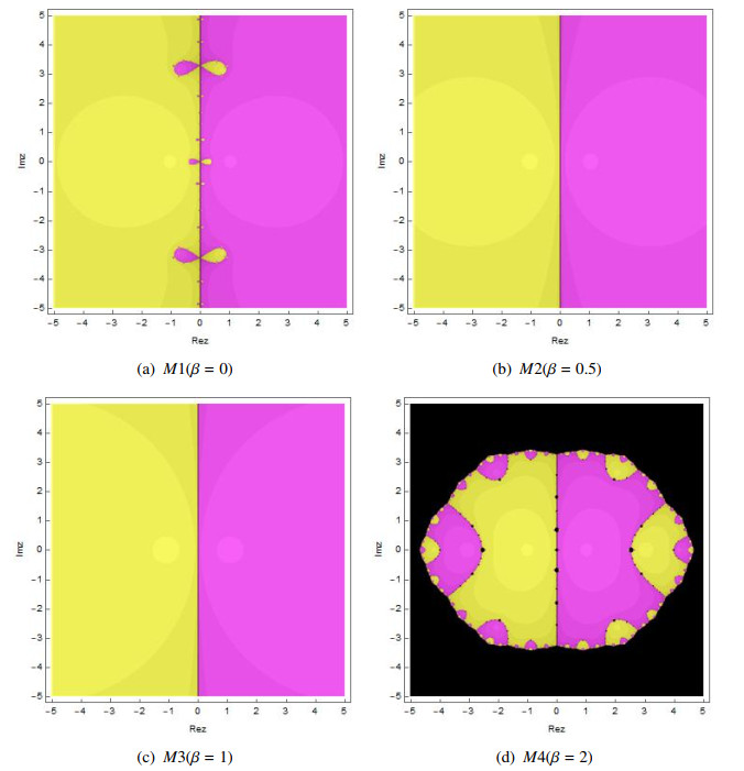
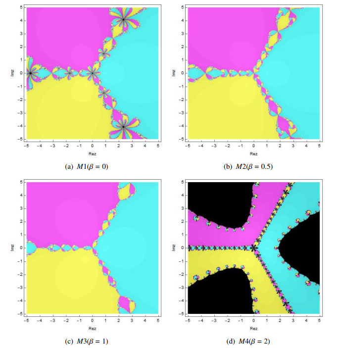
In this paper, the local convergence of a high-order Chebyshev-type method without the second derivative is studied. We study the convergence under $ \omega $-continuity conditions based on the first derivative. The uniqueness of the solution and the radii of convergence domains are obtained. In contrast to the conditions used in previous studies, the new conditions of convergence are weaker. In addition, the attractive basins of the family with different parameters are studied, which can show the different stability of the family. Finally, in numerical experiments, the iterative method is used to solve different nonlinear models, including vertical stresses, civil engineering problem, blood rheology model, and so on. Theoretical results of convergence criteria are verified.
Citation: Dongdong Ruan, Xiaofeng Wang. A high-order Chebyshev-type method for solving nonlinear equations: local convergence and applications[J]. Electronic Research Archive, 2025, 33(3): 1398-1413. doi: 10.3934/era.2025065
In this paper, the local convergence of a high-order Chebyshev-type method without the second derivative is studied. We study the convergence under $ \omega $-continuity conditions based on the first derivative. The uniqueness of the solution and the radii of convergence domains are obtained. In contrast to the conditions used in previous studies, the new conditions of convergence are weaker. In addition, the attractive basins of the family with different parameters are studied, which can show the different stability of the family. Finally, in numerical experiments, the iterative method is used to solve different nonlinear models, including vertical stresses, civil engineering problem, blood rheology model, and so on. Theoretical results of convergence criteria are verified.

| [1] | I. K. Argyros, The Theory and Applications of Iteration Methods, CRC Press, 2022. http://dx.doi.org/10.1201/9781003128915 |
| [2] | A. A. Samarskii, E.S. Nikolaev, The mathematical theory of iterative methods, Birkhäuser Basel, 1989. http://dx.doi.org/10.1007/978-3-0348-9142-4_1 |
| [3] |
I. K. Argyros, S. Hilout, Weaker conditions for the convergence of Newton's method, J. Complex., 28 (2012), 364–387. https://doi.org/10.1016/j.jco.2011.12.003 doi: 10.1016/j.jco.2011.12.003

|
| [4] | I. K. Argyros, Convergence and Application of Newton-type Iterations, Springer, 2008. http://dx.doi.org/10.1007/978-0-387-72741-7 |
| [5] |
X. Wang, W. Li, Fractal behavior of King's optimal eighth-order iterative method and its numerical application, Math. Commun., 9 (2024), 217–236. https://doi.org/10.3934/math.20231141 doi: 10.3934/math.20231141
|
| [6] |
X. Wang, N. Shang, Local convergence analysis of a novel derivative-free method with and without memory for solving nonlinear systems, Int. J. Comput. Math., (2025), 1–18. https://doi.org/10.1080/00207160.2025.2464701 doi: 10.1080/00207160.2025.2464701
|
| [7] | D. Ruan, X. Wang, Local convergence of seventh-order iterative method under weak conditions and its applications, Eng. Comput., 2025, In press. https://doi.org/10.1108/EC-08-2024-0775 |
| [8] |
I. K. Argyros, H. Ren, Improved local analysis for certain class of iterative methods with cubic convergence, Numer. Algorithms, 59 (2012), 505–521. https://doi.org/10.1007/s11075-011-9501-6 doi: 10.1007/s11075-011-9501-6
|
| [9] |
S. George, I. K. Argyros, Local convergence for a Chebyshev-type method in Banach space free of derivatives, Adv. Theory Nonlinear Anal. Appl., 2 (2018), 62–69. https://doi.org/10.31197/atnaa.400459 doi: 10.31197/atnaa.400459
|
| [10] |
X. Yang, Z. Zhang, Analysis of a new NFV scheme preserving DMP for two-dimensional sub-diffusion equation on distorted meshes, J. Sci. Comput., 99 (2024), 80. https://doi.org/10.1007/s10915-024-02511-7 doi: 10.1007/s10915-024-02511-7
|
| [11] |
X. Yang, Z. Zhang, Superconvergence analysis of a robust orthogonal Gauss collocation method for 2D fourth-order subdiffusion equations, J. Sci. Comput., 100 (2024), 62. https://doi.org/10.1007/s10915-024-02616-z doi: 10.1007/s10915-024-02616-z
|
| [12] |
K. Liu, Z. He, H. Zhang, X. Yang, A Crank–Nicolson ADI compact difference scheme for the three-dimensional nonlocal evolution problem with a weakly singular kernel, Comput. Appl. Math., 44 (2025), 164. https://doi.org/10.1007/s40314-025-03125-x doi: 10.1007/s40314-025-03125-x
|
| [13] |
W. Wang, H. Zhang, X. Jiang, X. Yang, A high-order and efficient numerical technique for the nonlocal neutron diffusion equation representing neutron transport in a nuclear reactor, Ann. Nucl. Energy, 195 (2024), 110163. https://doi.org/10.1016/j.anucene.2023.110163 doi: 10.1016/j.anucene.2023.110163
|
| [14] |
X. Wang, D. Ruan, Convergence ball of a new fourth-order method for finding a zero of the derivative, AIMS Math., 9 (2024), 6073–6087. https://doi.org/10.3934/math.2024297 doi: 10.3934/math.2024297
|
| [15] |
J. M. Gutiérrez, M. A. Hernández, A family of Chebyshev-Halley type methods in Banach spaces, Bull. Austral. Math. Soc., 55 (1997), 113–130. https://doi.org/10.1017/S0004972700030586 doi: 10.1017/S0004972700030586
|
| [16] |
J. A. Ezquerro, M.A. Hernández, On the R-order of the Halley method, J. Math. Anal. Appl., 303 (2005), 591–601. https://doi.org/10.1016/j.jmaa.2004.08.057 doi: 10.1016/j.jmaa.2004.08.057
|
| [17] |
M. A. Hernández, Chebyshev's approximation algorithms and applications, Comput. Math. Appl., 41 (2001), 433–455. https://doi.org/10.1016/S0898-1221(00)00286-8 doi: 10.1016/S0898-1221(00)00286-8
|
| [18] | M. S. Petković, B. Neta, L. D. Petković, J. Džunić, Multipoint Methods for Solving Nonlinear Equations, Elsevier, (2012), 281–291. https://doi.org/10.5555/2502628 |
| [19] |
D. Li, P. Liu, J. Kou, An improvement of Chebyshev-Halley methods free from second derivative, Appl. Math. Comput., 235 (2014), 221–225. https://doi.org/10.1016/j.amc.2014.02.083 doi: 10.1016/j.amc.2014.02.083
|
| [20] |
A. Cordero, T. Lotfi, K. Mahdiani, J. R. Torregrosa, A stable family with high order of convergence for solving nonlinear equations, Appl. Math. Comput., 254 (2015), 240–251. https://doi.org/10.1016/j.amc.2014.12.141 doi: 10.1016/j.amc.2014.12.141
|
| [21] |
P. Sivakumar, J. Jayaraman, Some new higher order weighted newton methods for solving nonlinear equation with applications, Math. Comput. Appl., 24(2) (2019), 59. https://doi.org/10.3390/mca24020059 doi: 10.3390/mca24020059
|
| [22] | S. Chapra, Applied Numerical Methods with MATLAB for Engineers and Scientists, McGraw Hill, 2011. https://doi.org/10.5555/1202863 |
| [23] |
M. Shams, N. Rafiq, N. Kausar, N. Mir, A. Alalyani, Computer oriented numerical scheme for solving engineering problems, Comput. Syst. Sci. Eng., 42 (2022), 689–701. https://doi.org/10.32604/csse.2022.022269 doi: 10.32604/csse.2022.022269
|
| [24] |
S. Qureshi, A. Soomro, A. A. Shaikh, E. Hincal, N. Gokbulut, A novel multistep iterative technique for models in medical sciences with complex dynamics, Comput. Math. Methods Med., 1 (2022), 7656451. https://doi.org/10.1155/2022/7656451 doi: 10.1155/2022/7656451
|
| [25] |
J. R. Sharma, S. Kumar, H. Singh, A new class of derivative-free root solvers with increasing optimal convergence order and their complex dynamics, SeMA J., 80 (2023), 333–352. https://doi.org/10.1007/s40324-022-00288-z doi: 10.1007/s40324-022-00288-z
|
| [26] |
A. Cordero, J. R. Torregrosa, Variants of Newton's Method using fifth-order quadrature formulas. Appl. Math. Comput., 190 (2007), 686-698. https://doi.org/10.1016/j.amc.2007.01.062 doi: 10.1016/j.amc.2007.01.062
|
Figures(2) / Tables(1)
Dongdong Ruan, Xiaofeng Wang. A high-order Chebyshev-type method for solving nonlinear equations: local convergence and applications[J]. Electronic Research Archive, 2025, 33(3): 1398-1413. doi: 10.3934/era.2025065


 DownLoad: