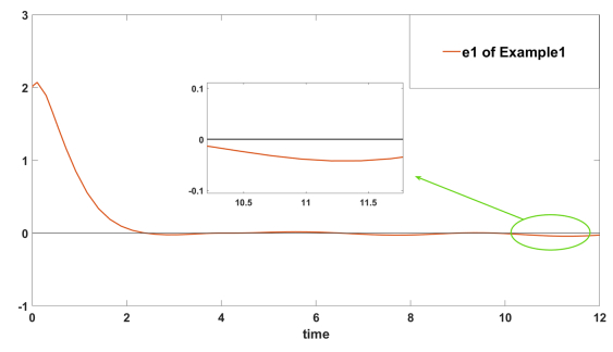
Previous works have analyzed finite/fixed-time tracking control for nonlinear systems. In these works, achieving the accurate time convergence of errors must be under the premise of known initial values and careful design of control parameters. Then, how to break through the constraints of initial values and design parameters for this issue is an unsolved problem. Motivated by this, we successfully studied prescribed-time tracking control for single-input single-output nonlinear systems with uncertainties. Specifically, we designed a state feedback controller on $ [0, {T}_{p}) $, based on the backstepping method, to make the tracking error (TE) tend to zero at $ {T}_{p} $, in which $ {T}_{p} $ is the arbitrarily selected prescribed-time. Furthermore, on $ [{T}_{p}, \mathrm{\infty }), $ another controller, similarly to that on $ [0, {T}_{p}) $, was designed to keep TE within a precision after $ {T}_{p} $, while TE may not stay at zero. Therefore, on $ [{T}_{p}, \mathrm{\infty }) $, another new controller, based on sliding mode control, was built to ensure that TE stays at zero after $ {T}_{p}. $
Citation: Lichao Feng, Chunlei Zhang, Mahmoud Abdel-Aty, Jinde Cao, Fawaz E. Alsaadi. Prescribed-time trajectory tracking control for a class of nonlinear system[J]. Electronic Research Archive, 2024, 32(12): 6535-6552. doi: 10.3934/era.2024305
Previous works have analyzed finite/fixed-time tracking control for nonlinear systems. In these works, achieving the accurate time convergence of errors must be under the premise of known initial values and careful design of control parameters. Then, how to break through the constraints of initial values and design parameters for this issue is an unsolved problem. Motivated by this, we successfully studied prescribed-time tracking control for single-input single-output nonlinear systems with uncertainties. Specifically, we designed a state feedback controller on $ [0, {T}_{p}) $, based on the backstepping method, to make the tracking error (TE) tend to zero at $ {T}_{p} $, in which $ {T}_{p} $ is the arbitrarily selected prescribed-time. Furthermore, on $ [{T}_{p}, \mathrm{\infty }), $ another controller, similarly to that on $ [0, {T}_{p}) $, was designed to keep TE within a precision after $ {T}_{p} $, while TE may not stay at zero. Therefore, on $ [{T}_{p}, \mathrm{\infty }) $, another new controller, based on sliding mode control, was built to ensure that TE stays at zero after $ {T}_{p}. $

| [1] | A. Y. Aleksandrov, E. B. Aleksandrova, A. P. Zhabko, On the asymptotic stability with respect to a part of variables of solutions of nonlinear systems with delay, in 2016 International Conference Stability and Oscillations of Nonlinear Control Systems, IEEE, (2016), 1–3. https://doi.org/10.1109/STAB.2016.7541155 |
| [2] |
M. Bucolo, A. Buscarino, L. Fortuna, S. Gagliano, A new asymptotic stability criterion for linear discrete-time systems, IEEE Trans. Circuits Syst. II Express Briefs, 69 (2022), 4994–4998. https://doi.org/10.1109/TCSII.2022.3187864 doi: 10.1109/TCSII.2022.3187864

|
| [3] |
F. Zhang, Z. Zeng, Asymptotic stability and synchronization of fractional-order neural networks with unbounded time-varying delays, IEEE Trans. Syst. Man Cybern.: Syst., 51 (2021), 5547–5556. https://doi.org/10.1109/TSMC.2019.2956320 doi: 10.1109/TSMC.2019.2956320
|
| [4] |
L. Feng, S. Li, X. Mao, Asymptotic stability and boundedness of stochastic functional differential equations with Markovian switching, J. Franklin Inst., 353 (2016), 4924–4949. https://doi.org/10.1016/j.jfranklin.2016.09.017 doi: 10.1016/j.jfranklin.2016.09.017
|
| [5] |
L. Feng, L. Liu, J. Cao, L. Rutkowski, G. Lu, General decay stability for non-autonomous neutral stochastic systems with time-varying delays and Markovian switching, IEEE Trans. Cybern., 52 (2022), 5441–5453. https://doi.org/10.1109/TCYB.2020.3031992 doi: 10.1109/TCYB.2020.3031992
|
| [6] |
H. Lin, H. Zeng, X. Zhang, W. Wang, Stability analysis for delayed neural networks via a generalized reciprocally convex inequality, IEEE Trans. Neural Networks Learn. Syst., 34 (2023), 7491–7499. https://doi.org/10.1109/TNNLS.2022.3144032 doi: 10.1109/TNNLS.2022.3144032
|
| [7] |
T. Peng, H. Zeng, W. Wang, X. Zhang, X. Liu, General and less conservative criteria on stability and stabilization of T–S fuzzy systems with time-varying delay, IEEE Trans. Fuzzy Syst., 31 (2023), 1531–1541. https://doi.org/10.1109/TFUZZ.2022.3204899 doi: 10.1109/TFUZZ.2022.3204899
|
| [8] |
L. Weiss, E. Infante, Finite time stability under perturbing forces and on product spaces, IEEE Trans. Autom. Control, 12 (1967), 54–59. https://doi.org/10.1109/TAC.1967.1098483 doi: 10.1109/TAC.1967.1098483
|
| [9] |
Y. Wu, X. Yu, Z. Man, Terminal sliding mode control design for uncertain dynamic systems, Syst. Control Lett., 34 (1998), 281–287. https://doi.org/10.1016/S0167-6911(98)00036-X doi: 10.1016/S0167-6911(98)00036-X
|
| [10] |
A. Levant, Homogeneity approach to high-order sliding mode design, Automatica, 41 (2005), 823–830. https://doi.org/10.1016/j.automatica.2004.11.029 doi: 10.1016/j.automatica.2004.11.029
|
| [11] |
M. Chen, Q. Wu, R. Cui, Terminal sliding mode tracking control for a class of SISO uncertain nonlinear systems, ISA Trans., 52 (2013), 198–206. https://doi.org/10.1016/j.isatra.2012.09.009 doi: 10.1016/j.isatra.2012.09.009
|
| [12] |
S. Bhat, D. Bernstein, Finite-time stability of continuous autonomous systems, SIAM J. Control Optim., 38 (2000), 751–766. https://doi.org/10.1137/S0363012997321358 doi: 10.1137/S0363012997321358
|
| [13] |
Y. Shen, Y. Huang, Global finite-time stabilisation for a class of nonlinear systems, Int. J. Syst. Sci., 43 (2012), 73–78. https://doi.org/10.1080/00207721003770569 doi: 10.1080/00207721003770569
|
| [14] |
M. Ahmad, M. Akram, M. Mohsan, K. Saghar, R. Ahmad, W. Butt, Transformer-based sensor failure prediction and classification framework for UAVs, Expert Syst. Appl., 248 (2024), 123415. https://doi.org/10.1016/j.eswa.2024.123415 doi: 10.1016/j.eswa.2024.123415
|
| [15] |
A. Polyakov, Nonlinear feedback design for fixed-time stabilization of linear control systems, IEEE Trans. Autom. Control, 57 (2012), 2106–2110. https://doi.org/10.1109/TAC.2011.2179869 doi: 10.1109/TAC.2011.2179869
|
| [16] |
C. Chen, Z. Sun, Fixed-time stabilisation for a class of high order non-linear systems, IET Control Theory Appl., 12 (2018), 2578–2587. https://doi.org/10.1049/iet-cta.2018.5053 doi: 10.1049/iet-cta.2018.5053
|
| [17] |
B. Ning, Q. L. Han, Z. Zuo, L. Ding, Q. Lu, X. Ge, Fixed-time and prescribed-time consensus control of multi-agent systems and its applications: A survey of recent trends and methodologies, IEEE Trans. Ind. Inf., 19 (2023), 1121–1135. https://doi.org/10.1109/TII.2022.3201589 doi: 10.1109/TII.2022.3201589
|
| [18] |
Y. Song, Y. Wang, J. Holloway, M. Krstic, Time-varying feedback for regulation of normal-form nonlinear systems in prescribed finite time, Automatica, 83 (2017), 243–251. https://doi.org/10.1016/j.automatica.2017.06.008 doi: 10.1016/j.automatica.2017.06.008
|
| [19] |
J. Holloway, M. Krstic, Prescribed-time observers for linear systems in observer canonical form, IEEE Trans. Autom. Control, 64 (2019), 3905–3912. https://doi.org/10.1109/TAC.2018.2890751 doi: 10.1109/TAC.2018.2890751
|
| [20] |
N. Espitia, D. Steeves, W. Perruquetti, M. Krstic, Sensor delay compensated prescribed-time observer for LTI systems, Automatica, 135 (2022), 110005. https://doi.org/10.1016/j.automatica.2021.110005 doi: 10.1016/j.automatica.2021.110005
|
| [21] |
H. Ye, Y. Song, Prescribed-time control for linear systems in canonical form via nonlinear feedback, IEEE Trans. Syst. Man Cybern.: Syst., 53 (2023), 1126–1135. https://doi.org/10.1109/TSMC.2022.3194908 doi: 10.1109/TSMC.2022.3194908
|
| [22] |
A. K. Pal, S. Kamal, S. K. Nagar, B. Bandyopadhyay, L. Fridman, Design of controllers with arbitrary convergence time, Automatica, 112 (2020), 108710. https://doi.org/10.1016/j.automatica.2019.108710 doi: 10.1016/j.automatica.2019.108710
|
| [23] |
B. Zhou, Finite-time stability analysis and stabilization by bounded linear time-varying feedback, Automatica, 121 (2020), 109191. https://doi.org/10.1016/j.automatica.2020.109191 doi: 10.1016/j.automatica.2020.109191
|
| [24] |
B. Zhou, Y. Shi, Prescribed-time stabilization of a class of nonlinear systems by linear time-varying feedback, IEEE Trans. Autom. Control, 66 (2021), 6123–6130. https://doi.org/10.1109/TAC.2021.3061645 doi: 10.1109/TAC.2021.3061645
|
| [25] |
Z. Chen, X. Ju, Z. Wang, Q. Li, The prescribed time sliding mode control for attitude tracking of spacecraft, Asian J. Control, 24 (2022), 1650–1662. https://doi.org/10.1002/asjc.2569 doi: 10.1002/asjc.2569
|
| [26] |
D. Tran, T. Yucelen, Finite-time control of perturbed dynamical systems based on a generalized time transformation approach, Syst. Control Lett., 136 (2020), 104605. https://doi.org/10.1016/j.sysconle.2019.104605 doi: 10.1016/j.sysconle.2019.104605
|
| [27] |
C. Hua, P. Ning, K. Li, Adaptive prescribed-time control for a class of uncertain nonlinear systems, IEEE Trans. Autom. Control, 67 (2022), 6159–6166. https://doi.org/10.1109/TAC.2021.3130883 doi: 10.1109/TAC.2021.3130883
|
| [28] |
C. Hua, H. Li, K. Li, P. Ning, Adaptive prescribed-time control of time-delay nonlinear systems via a double time-varying gain approach, IEEE Trans. Cybern., 53 (2023), 5290–5298. https://doi.org/10.1109/TCYB.2022.3192250 doi: 10.1109/TCYB.2022.3192250
|
| [29] |
Y. Song, J. Su, A unified Lyapunov characterization for finite time control and prescribed time control, Int. J. Robust Nonlinear Control, 33 (2021), 2930–2949. https://doi.org/10.1002/rnc.6544 doi: 10.1002/rnc.6544
|
| [30] |
H. F. Ye, Y. D. Song, Prescribed-time control of uncertain strict-feedback-like systems, Int. J. Robust Nonlinear Control., 31 (2021), 5281–5297. https://doi.org/10.1002/rnc.5541 doi: 10.1002/rnc.5541
|
| [31] | Y. Cao, Y. D. Song, Practical prescribed time tracking control with user pre-determinable precision for uncertain nonlinear systems, in 2020 59th IEEE Conference on Decision and Control (CDC), IEEE, (2020), 3526–3530. https: //doi.org/10.1109/CDC42340.2020.9304143 |
| [32] |
R. Ma, L. Fu, J. Fu, Prescribed-time tracking control for nonlinear systems with guaranteed performance, Automatica, 146 (2022), 110573. https://doi.org/10.1016/j.automatica.2022.110573 doi: 10.1016/j.automatica.2022.110573
|
| [33] |
Y. Li, R. Ma, X. Tian, Prescribed-time tracking with prescribed performance for a class of strict-feedback nonlinear systems, J. Franklin Inst., 361 (2024), 106638. https://doi.org/10.1016/j.jfranklin.2024.01.039 doi: 10.1016/j.jfranklin.2024.01.039
|
| [34] | H. K. Khalil, Nonlinear Systems (3rd edition), Prentice-Hal, 2002. |
| [35] |
H. Wang, B. Su, Y. Wang, J. Gao, Adaptive sliding mode fixed-time tracking control based on fixed-time sliding mode disturbance observer with dead-zone input, Complexity, 2019 (2019), 8951382. https://doi.org/10.1155/2019/8951382 doi: 10.1155/2019/8951382
|
| [36] |
M. Chen, Y. Li, H. Wang, K. Peng, L. Wu, Adaptive fixed-time tracking control for nonlinear systems based on finite-time command-filtered backstepping, IEEE Trans. Fuzzy Syst., 31 (2023), 1604–1613. https://doi.org/10.1109/TFUZZ.2022.3206507 doi: 10.1109/TFUZZ.2022.3206507
|
| [37] |
D. Cui, M. Chali, Z. Xiang, Fuzzy fault-tolerant predefined-time control for switched systems: A singularity-free method, IEEE Trans. Fuzzy Syst., 32 (2024), 1223–1232. https://doi.org/10.1109/TFUZZ.2023.3321688 doi: 10.1109/TFUZZ.2023.3321688
|
| [38] |
Y. Song, H. Ye, F. Lewis, Prescribed-time control and its latest developments, IEEE Trans. Syst. Man Cybern.: Syst., 53 (2023), 4102–4116. https://doi.org/10.1109/TSMC.2023.3240751 doi: 10.1109/TSMC.2023.3240751
|
| [39] |
D. Cui, C. K. Ahn, Y. Sun, Z. Xiang, Mode-dependent state observer-based prescribed performance control of switched systems, IEEE Trans. Circuits Syst. II Express Briefs, 71 (2024), 3810–3814. https://doi.org/10.1109/TCSII.2024.3370865 doi: 10.1109/TCSII.2024.3370865
|
| [40] |
H. Zeng, Z. Zhu, T. Peng, W. Wang, X. Zhang, Robust tracking control design for a class of nonlinear networked control systems considering bounded package dropouts and external disturbance, IEEE Trans. Fuzzy Syst., 32 (2024), 3608–3617. https://doi.org/10.1109/TFUZZ.2024.3377799 doi: 10.1109/TFUZZ.2024.3377799
|


Figures(8)
Lichao Feng, Chunlei Zhang, Mahmoud Abdel-Aty, Jinde Cao, Fawaz E. Alsaadi. Prescribed-time trajectory tracking control for a class of nonlinear system[J]. Electronic Research Archive, 2024, 32(12): 6535-6552. doi: 10.3934/era.2024305


 DownLoad: