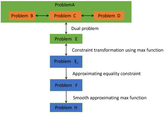
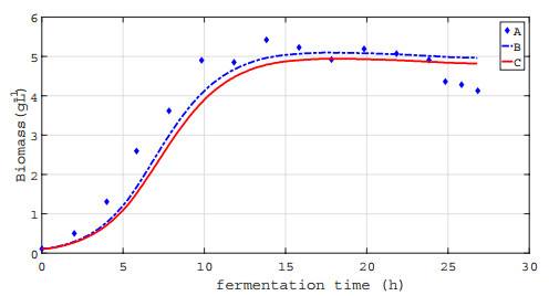
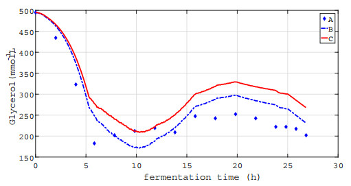
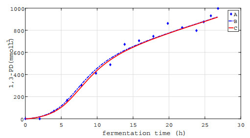
In this paper, we investigated a nonlinear continuous-time switched time-delay (NCTSTD) system for glycerol fed-batch bioconversion to 1, 3-propanediol with unknown time-delay and system parameters. The measured output data was uncertain, while the first moment information about its distribution was available. Our goal was to identify these unknown quantities under the environment of uncertain measurement output data. A distributionally robust parameter estimation problem (i.e., a bi-level parameter estimation (BLPE) problem) subject to the NCTSTD system was presented, where the expectation of the discrepancy between the output of the NCTSTD system and the uncertain measured output data with respect to its probability distributions was included in the cost functional. By applying the duality theory, the BLPE problem was transformed into a single-level parameter estimation (SLPE) problem with non-smooth term approximated by a smoothing technique and its error analysis was given. Then, the gradients of the cost function of the SLPE problem were derived. A hybrid optimization algorithm was proposed for solving the SLPE problem. The paper concluded by presenting the simulation results.
Citation: Sida Lin, Jinlong Yuan, Zichao Liu, Tao Zhou, An Li, Chuanye Gu, Kuikui Gao, Jun Xie. Distributionally robust parameter estimation for nonlinear fed-batch switched time-delay system with moment constraints of uncertain measured output data[J]. Electronic Research Archive, 2024, 32(10): 5889-5913. doi: 10.3934/era.2024272
In this paper, we investigated a nonlinear continuous-time switched time-delay (NCTSTD) system for glycerol fed-batch bioconversion to 1, 3-propanediol with unknown time-delay and system parameters. The measured output data was uncertain, while the first moment information about its distribution was available. Our goal was to identify these unknown quantities under the environment of uncertain measurement output data. A distributionally robust parameter estimation problem (i.e., a bi-level parameter estimation (BLPE) problem) subject to the NCTSTD system was presented, where the expectation of the discrepancy between the output of the NCTSTD system and the uncertain measured output data with respect to its probability distributions was included in the cost functional. By applying the duality theory, the BLPE problem was transformed into a single-level parameter estimation (SLPE) problem with non-smooth term approximated by a smoothing technique and its error analysis was given. Then, the gradients of the cost function of the SLPE problem were derived. A hybrid optimization algorithm was proposed for solving the SLPE problem. The paper concluded by presenting the simulation results.

| [1] |
W. Liu, L. Yang, B. Yu, Kernel density estimation based distributionally robust mean-CVaR portfolio optimization, J. Glob. Optim., 84 (2022), 1053–1077. https://doi.org/10.1007/s10898-022-01177-5 doi: 10.1007/s10898-022-01177-5

|
| [2] |
E. Delage, Y. Ye, Distributionally robust optimization under moment uncertainty with application to data-driven problems, Oper. Res., 58 (2010), 595–612. https://doi.org/10.1287/opre.1090.0741 doi: 10.1287/opre.1090.0741
|
| [3] |
C. Peng, E. Delage, Data-driven optimization with distributionally robust second order stochastic dominance constraints, Oper. Res., 72 (2024), 1298–1316. https://doi.org/10.1287/opre.2022.2387 doi: 10.1287/opre.2022.2387
|
| [4] |
S. Wang, L. Pang, H. Guo, H. Zhang, Distributionally robust optimization with multivariate second-order stochastic dominance constraints with applications in portfolio optimization, Optimization, 72 (2023), 1839–1862. https://doi.org/10.1080/02331934.2022.2048382 doi: 10.1080/02331934.2022.2048382
|
| [5] |
X. Tong, M. Li, H. Sun, Decision bounding problems for two-stage distributionally robust stochastic bilevel optimization, J. Glob. Optim., 87 (2023), 679–707. https://doi.org/10.1007/s10898-022-01227-y doi: 10.1007/s10898-022-01227-y
|
| [6] |
H. Xu, Y. Liu, H. Sun, Distributionally robust optimization with matrix moment constraints: Lagrange duality and cutting plane methods, Math. Program., 169 (2018), 489–529. https://doi.org/10.1007/s10107-017-1143-6 doi: 10.1007/s10107-017-1143-6
|
| [7] |
B. Li, Y. Rong, J. Sun, K. L. Teo, A distributionally robust linear receiver design for multi-access space-time block coded MIMO systems, IEEE Trans. Wireless Commun., 16 (2017), 464–474. https://doi.org/10.1109/TWC.2016.2625246 doi: 10.1109/TWC.2016.2625246
|
| [8] |
B. Li, Y. Tan, A. Wu, G. Duan, A distributionally robust optimization based method for stochastic model predictive control, IEEE Trans. Autom. Control, 67 (2022), 5762–5776. https://doi.org/10.1109/TAC.2021.3124750 doi: 10.1109/TAC.2021.3124750
|
| [9] |
A. Shapiro, Distributionally robust modeling of optimal control, Oper. Res. Lett., 50 (2022), 561–567. https://doi.org/10.1016/j.orl.2022.08.002 doi: 10.1016/j.orl.2022.08.002
|
| [10] |
B. P. Van Parys, D. Kuhn, P. J. Goulart, M. Morari, Distributionally robust control of constrained stochastic systems, IEEE Trans. Autom. Control, 61 (2015), 430–442. https://doi.org/10.1109/TAC.2015.2444134 doi: 10.1109/TAC.2015.2444134
|
| [11] |
A. Hakobyan, I. Yang, Wasserstein distributionally robust control of partially observable linear stochastic systems, IEEE Trans. Autom. Control, 69 (2024), 6121–6136. https://doi.org/10.1109/TAC.2024.3394348 doi: 10.1109/TAC.2024.3394348
|
| [12] | B. Li, T. Guan, L. Dai, G. R. Duan. Distributionally robust model predictive control with output feedback. IEEE Trans. Autom. Control, 69 (2024), 3270–3277. https://doi.org/10.1109/TAC.2023.3321375 |
| [13] |
L. Huang, X. Zhou, N. Wu, Y. Sun, Z. Xiu, Selective extraction of 1, 3-propanediol by phenylboronic acid-based ternary extraction system, J. Chem. Technol. Biotechnol., 99 (2024), 1530–1540. https://doi.org/10.1002/jctb.7647 doi: 10.1002/jctb.7647
|
| [14] |
C. Groeger, W. Sabra, A. Zeng, Simultaneous production of 1, 3-propanediol and n-butanol by Clostridium pasteurianum: In situ gas stripping and cellular metabolism, Eng. Life Sci., 16 (2016), 664–674. https://doi.org/10.1002/elsc.201600058 doi: 10.1002/elsc.201600058
|
| [15] |
J. Zhou, J. Shen, X. Wang, Y. Sun, Z. Xiu, Metabolism, morphology and transcriptome analysis of oscillatory behavior of Clostridium butyricum during long-term continuous fermentation for 1, 3-propanediol production, Biotechnol. Biofuels, 13 (2020), 191. https://doi.org/10.1186/s13068-020-01831-8 doi: 10.1186/s13068-020-01831-8
|
| [16] |
S. Duan, Z. Zhang, X. Wang, Y. Sun, Y. Dong, L. Ren, et al., Co-production of 1, 3-propanediol and phage phiKpS2 from the glycerol fermentation by Klebsiella pneumoniae, Bioresour. Bioprocess., 11 (2024), 44. https://doi.org/10.1186/s40643-024-00760-w doi: 10.1186/s40643-024-00760-w
|
| [17] |
L. Wang, J. Yuan, C. Wu, X. Wang, Practical algorithm for stochastic optimal control problem about microbial fermentation in batch culture, Optim. Lett., 13 (2019), 527–541. https://doi.org/10.1007/s11590-017-1220-z doi: 10.1007/s11590-017-1220-z
|
| [18] |
J. Wang, X. Zhang, J. Ye, J. Wang, E. Feng, Optimizing design for continuous conversion of glycerol to 1, 3-propanediol using discrete-valued optimal control, J. Process Control, 104 (2021), 126–134. https://doi.org/10.1016/j.jprocont.2021.06.010 doi: 10.1016/j.jprocont.2021.06.010
|
| [19] |
J. Yuan, S. Lin, S. Zhang, C. Liu, Distributionally robust system identification for continuous fermentation nonlinear switched system under moment uncertainty of experimental data, Appl. Math. Modell., 127 (2024), 679–695. https://doi.org/10.1016/j.apm.2023.12.023 doi: 10.1016/j.apm.2023.12.023
|
| [20] |
J. Yuan, C. Wu, C. Liu, K. L. Teo, J. Xie, Robust suboptimal feedback control for a fed-batch nonlinear time-delayed switched system, J. Franklin Inst., 360 (2023), 1835–1869. https://doi.org/10.1016/j.jfranklin.2022.12.027 doi: 10.1016/j.jfranklin.2022.12.027
|
| [21] |
C. Liu, G. Shi, G. Liu, D. Hu, Optimal control of a nonlinear state-dependent impulsive system in fed-batch process, Int. J. Biomath., 16 (2023), 2350001. https://doi.org/10.1142/S1793524523500018 doi: 10.1142/S1793524523500018
|
| [22] |
T. Niu, J. Zhai, H. Yin, E. Feng, C. Liu, The uncoupled microbial fed-batch fermentation optimization based on state-dependent switched system, Int. J. Biomath., 14 (2021), 2150025. https://doi.org/10.1142/S179352452150025X doi: 10.1142/S179352452150025X
|
| [23] |
X. Li, M. Sun, Z. Gong, E. Feng, Multistage optimal control for microbial fed-batch fermentation process, J. Ind. Manage. Optim., 18 (2022), 1709–1721. https://doi.org/10.3934/jimo.2021040 doi: 10.3934/jimo.2021040
|
| [24] |
T. Niu, J. Zhai, H. Yin, E. Feng, Optimal control of nonlinear switched system in an uncoupled microbial fed-batch fermentation process, J. Franklin Inst., 355 (2018), 6169–6190. https://doi.org/10.1016/j.jfranklin.2018.05.012 doi: 10.1016/j.jfranklin.2018.05.012
|
| [25] |
C. Zhang, S. Sharma, W. Wang, A. Zeng, A novel downstream process for highly pure 1, 3-propanediol from an efficient fed-batch fermentation of raw glycerol by Clostridium pasteurianum, Eng. Life Sci., 21 (2021), 351–363. https://doi.org/10.1002/elsc.202100012 doi: 10.1002/elsc.202100012
|
| [26] |
J. Yuan, S. Zhao, D. Yang, C. Liu, C. Wu, T. Zhou, et al., Koopman modeling and optimal control for microbial fed-batch fermentation with switching operators, Nonlinear Anal. Hybrid Syst., 52 (2024), 101461. https://doi.org/10.1016/j.nahs.2023.101461 doi: 10.1016/j.nahs.2023.101461
|
| [27] |
J. Yuan, C. Wu, Z. Liu, S. Zhao, C. Yu, K. Teo, et al., Koopman modeling for optimal control of the perimeter of multi-region urban traffic networks, Appl. Math. Modell., 138 (2025), 115742. https://doi.org/10.1016/j.apm.2024.115742 doi: 10.1016/j.apm.2024.115742
|
| [28] |
D. Wu, Y. Bai, C. Yu, A new computational approach for optimal control problems with multiple time-delay, Automatica, 101 (2019), 388–395. https://doi.org/10.1016/j.automatica.2018.12.036 doi: 10.1016/j.automatica.2018.12.036
|
| [29] |
M. Wang, N. Liu, Qualitative analysis and traveling wave solutions of a predator-prey model with time delay and stage structure, Electron. Res. Arch., 32 (2024), 2665–2698. https://doi.org/10.3934/era.2024121 doi: 10.3934/era.2024121
|
| [30] |
J. Yuan, C. Wu, K. Teo, S. Zhao, L. Meng, Perimeter control with state-dependent delays: optimal control model and computational method, IEEE Trans. Intell. Transp. Syst., 23 (2022), 20614–20627. https://doi.org/10.1109/TITS.2022.3179729 doi: 10.1109/TITS.2022.3179729
|
| [31] |
D. Wu, Y. Chen, C. Yu, Y. Bai, K. Teo, Control parameterization approach to time-delay optimal control problems: A survey, J. Ind. Manage. Optim., 19 (2023), 3750–3783. https://doi.org/10.3934/jimo.2022108 doi: 10.3934/jimo.2022108
|
| [32] |
Y. Chen, X. Zhu, C. Yu, K. Teo, Sequential time scaling transformation technique for time-delay optimal control problem, Commun. Nonlinear Sci. Numer. Simul., 133 (2024), 107988. https://doi.org/10.1016/j.cnsns.2024.107988 doi: 10.1016/j.cnsns.2024.107988
|
| [33] | Z. Li, L. Pei, G. Duan, S. Chen, A non-autonomous time-delayed SIR model for COVID-19 epidemics prediction in China during the transmission of Omicron variant. Electron. Res. Arch., 32 (2024), 2203–2228. https://doi.org/10.3934/era.2024100 |
| [34] |
J. Yuan, C. Wu, K. Teo, J. Xie, S. Wang, Computational method for feedback perimeter control of multiregion urban traffic networks with state-dependent delays, Transp. Res. Part C Emerging Technol., 153 (2023), 104231. https://doi.org/10.1016/j.trc.2023.104231 doi: 10.1016/j.trc.2023.104231
|
| [35] | J. Yuan, D. Yang, D. Xun, K. Teo, C. Wu, A. Li, et al., Sparse optimal control of cyber-physical systems via PQA approach, Pac. J. Optim., Accepted, 2024. |
| [36] |
C. Liu, R. Ryan, Q. Lin, K. Teo, Dynamic optimization for switched time-delay systems with state-dependent switching conditions, SIAM J. Control Optim., 56 (2018), 3499–3523. https://doi.org/10.1137/16M1070530 doi: 10.1137/16M1070530
|
| [37] |
C. Liu, C. Sun, Robust parameter identification of a nonlinear impulsive time-delay system in microbial fed-batch process, Appl. Math. Modell., 111 (2022), 160–175. https://doi.org/10.1016/j.apm.2022.06.032 doi: 10.1016/j.apm.2022.06.032
|
| [38] |
X. Gao, J. Zhai, E. Feng, Multi-objective optimization of a nonlinear switched time-delay system in microbial fed-batch process, J. Franklin Inst., 357 (2020), 12609–12639. https://doi.org/10.1016/j.jfranklin.2020.07.036 doi: 10.1016/j.jfranklin.2020.07.036
|
| [39] |
C. Liu, M. Han, Time-delay optimal control of a fed-batch production involving multiple feeds, Discrete Contin. Dyn. Syst. - S, 13 (2020), 1697–1709. https://doi.org/10.3934/dcdss.2020099 doi: 10.3934/dcdss.2020099
|
| [40] | J. Nocedal, S. J. Wright, Numerical Optimization, Springer, New York, 2006. https://doi.org/10.1007/978-0-387-40065-5 |
| [41] |
A. Banerjee, I. Abu-Mahfouz, A comparative analysis of particle swarm optimization and differential evolution algorithms for parameter estimation in nonlinear dynamic systems, Chaos, Solitons Fractals, 58 (2014), 65–83. https://doi.org/10.1016/j.chaos.2013.11.004 doi: 10.1016/j.chaos.2013.11.004
|
| [42] | E. Anderson, P. Nash, Linear Programming in Infinite-Dimensional Spaces: Theory and Applications, Wiley, Chichester, United Kingdom, 1987. https://cir.nii.ac.jp/crid/1130000796325253632 |
| [43] |
C. Liu, Sensitivity analysis and parameter identification for a nonlinear time-delay system in microbial fed-batch process, Appl. Math. Modell., 38 (2014), 1449–1463. https://doi.org/10.1016/j.apm.2013.07.039 doi: 10.1016/j.apm.2013.07.039
|
| [44] |
P. Liu, X. Li, X. Liu, Y. Hu, An improved smoothing technique-based control vector parameterization method for optimal control problems with inequality path constraints, Optim. Control. Appl. Methods, 38 (2017), 586–600. https://doi.org/10.1002/oca.2273 doi: 10.1002/oca.2273
|
| [45] |
X. Wu, J. Lin, K. Zhang, M. Cheng, A penalty function-based random search algorithm for optimal control of switched systems with stochastic constraints and its application in automobile test-driving with gear shifts, Nonlinear Anal. Hybrid Syst., 45 (2022), 101218. https://doi.org/10.1016/j.nahs.2022.101218 doi: 10.1016/j.nahs.2022.101218
|
| [46] | K. Teo, B. Li, C. Yu, V. Rehbock, Applied and Computational Optimal Control: A Control Parametrization Approach, Springer, 2021. https://doi.org/10.1007/978-3-030-69913-0 |
| [47] |
X. Chen, D. J. Zhang, W. Qi, S. Gao, Z. Xiu, P. Xu, Microbial fed-batch production of 1, 3-propanediol by klebsiella pneumoniae under microaerobic conditions, Appl. Microbiol. Biotechnol., 63 (2003), 143–146. https://doi.org/10.1007/s00253-003-1369-5 doi: 10.1007/s00253-003-1369-5
|
| [48] | K. Atkinson, W. Han, D. Stewart, Numerical Solution of Ordinary Differential Equations, John Wiley and Sons, 2009. http://homepage.math.uiowa.edu/atkinson/papers/NAODE_Book.pdf |
Figures(4) / Tables(2)
Sida Lin, Jinlong Yuan, Zichao Liu, Tao Zhou, An Li, Chuanye Gu, Kuikui Gao, Jun Xie. Distributionally robust parameter estimation for nonlinear fed-batch switched time-delay system with moment constraints of uncertain measured output data[J]. Electronic Research Archive, 2024, 32(10): 5889-5913. doi: 10.3934/era.2024272


 DownLoad: