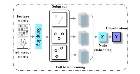
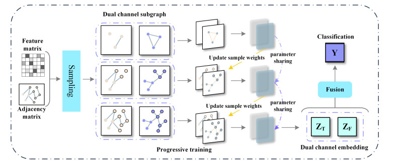
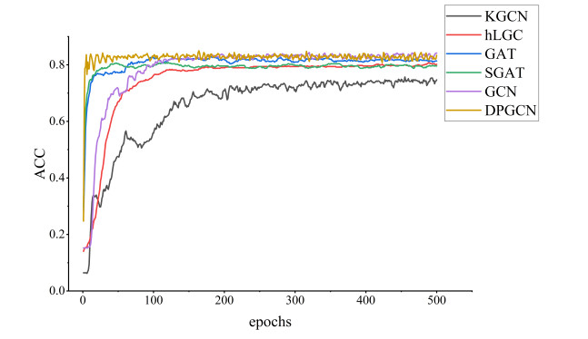
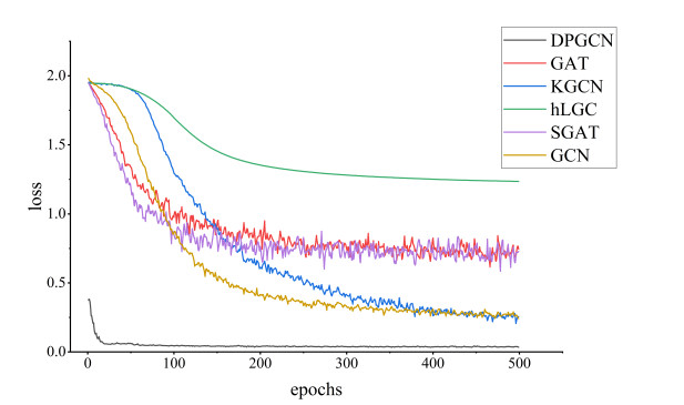
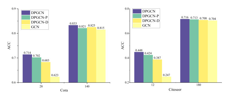
Graph Convolutional Networks (GCNs) demonstrate an excellent performance in node classification tasks by updating node representation via aggregating information from the neighbor nodes. Note that the complex interactions among all the nodes can produce challenges for GCNs. Independent subgraph sampling effectively limits the neighbor aggregation in convolutional computations, and it has become a popular method to improve the efficiency of training GCNs. However, there are still some improvements in the existing subgraph sampling strategies: 1) a loss of the model performance caused by ignoring the connection information among different subgraphs; and 2) a lack of representation power caused by an incomplete topology. Therefore, we propose a novel model called Dual-channel Progressive Graph Convolutional Network (DPGCN) via sub-graph sampling. We construct subgraphs via clustering and maintain the connection information among the different subgraphs. To enhance the representation power, we construct a dual channel fusion module by using both the geometric information of the node feature and the original topology. Specifically, we evaluate the complementary information of the dual channels based on the joint entropy between the feature information and the adjacency matrix, and effectively reduce the information redundancy by reasonably selecting the feature information. Then, the model convergence is accelerated through parameter sharing and weight updating in progressive training. We select 4 real datasets and 8 characteristic models for comparison on the semi-supervised node classification task. The results verify that the DPGCN possesses superior classification accuracy and robustness. In addition, the proposed architecture performs excellently in the low labeling rate, which is of practical value to label scarcity problems in real cases.
Citation: Wenrui Guan, Xun Wang. A Dual-channel Progressive Graph Convolutional Network via subgraph sampling[J]. Electronic Research Archive, 2024, 32(7): 4398-4415. doi: 10.3934/era.2024198
Graph Convolutional Networks (GCNs) demonstrate an excellent performance in node classification tasks by updating node representation via aggregating information from the neighbor nodes. Note that the complex interactions among all the nodes can produce challenges for GCNs. Independent subgraph sampling effectively limits the neighbor aggregation in convolutional computations, and it has become a popular method to improve the efficiency of training GCNs. However, there are still some improvements in the existing subgraph sampling strategies: 1) a loss of the model performance caused by ignoring the connection information among different subgraphs; and 2) a lack of representation power caused by an incomplete topology. Therefore, we propose a novel model called Dual-channel Progressive Graph Convolutional Network (DPGCN) via sub-graph sampling. We construct subgraphs via clustering and maintain the connection information among the different subgraphs. To enhance the representation power, we construct a dual channel fusion module by using both the geometric information of the node feature and the original topology. Specifically, we evaluate the complementary information of the dual channels based on the joint entropy between the feature information and the adjacency matrix, and effectively reduce the information redundancy by reasonably selecting the feature information. Then, the model convergence is accelerated through parameter sharing and weight updating in progressive training. We select 4 real datasets and 8 characteristic models for comparison on the semi-supervised node classification task. The results verify that the DPGCN possesses superior classification accuracy and robustness. In addition, the proposed architecture performs excellently in the low labeling rate, which is of practical value to label scarcity problems in real cases.

| [1] | L. F. R. Ribeiro, P. H. P. Saverese, D. R. Figueiredo, Struc2vec: Learning node representation from structural identity, in KDD '17 KDD '17: The 23rd ACM SIGKDD International Conference on Knowledge Discovery and Data Mining, ACM, (2017), 385–394. https://doi.org/10.1145/3097983.3098061 |
| [2] | Y. Zhang, S. Pal, M. Coates, D. Ustebay, Bayesian graph convolutional neural networks for semi-supervised classification, in Proceedings of the AAAI conference on artificial intelligence, AAAI, 33 (2019), 5829–5836. https://doi.org/10.1609/aaai.v33i01.33015829 |
| [3] | T. N. Kipf, M. Welling, Semi-supervised classification with graph convolutional networks, preprint, arXiv: 1609.02907. |
| [4] | N. Yadati, V. Nitin, M. Nimishakavi, P. Yadav, A. Louis, P. Talukdar, et al., NHP: Neural hypergraph link prediction, in CIKM '20: The 29th ACM International Conference on Information and Knowledge Management, ACM, (2020), 1705–1714. https://doi.org/10.1145/3340531.3411870 |
| [5] | D. Wang, P. Cui, W. Zhu, Structural deep network embedding, in KDD '16: Proceedings of the 22nd ACM SIGKDD International Conference on Knowledge Discovery and Data Mining, ACM, (2016), 1225–1234. https://doi.org/10.1145/2939672.2939753 |
| [6] |
S. Zhang, H. Tong, J. Xu, R. Maciejewski, Graph convolutional networks: A comprehensive review, Comput. Soc. Netw., 6 (2019), 11. https://doi.org/10.1186/s40649-019-0069-y doi: 10.1186/s40649-019-0069-y

|
| [7] |
X. X. Wang, X. B. Yang, P. X. Wang, H. L. Yu, T. H. Xu, SSGCN: A sampling sequential guided graph convolutional network, Int. J. Mach. Learn. Cyb., 15 (2024), 2023–2038. https://doi.org/10.1007/s13042-023-02013-2 doi: 10.1007/s13042-023-02013-2
|
| [8] | H. Q. Zeng, H. K. Zhou, A. Srivastava, R. Kannan, V. Prasanna, GraphSAINT: Graph sampling based inductive learning method, preprint, arXiv: 1907.04931. |
| [9] |
Q. Zhang, Y. F. Sun, Y. L. Hu, S. F. Wang, B. C. Yin, A subgraph sampling method for training large-scale graph convolutional network, Inf. Sci., 649 (2023), 119661. https://doi.org/10.1016/j.ins.2023.119661 doi: 10.1016/j.ins.2023.119661
|
| [10] |
S. T. Zhong, L. Huang, C. D. Wang, J. H. Lai, P. S. Yu, An autoencoder framework with attention mechanism for cross-domain recommendation, IEEE Trans. Cybern., 52 (2020), 5229–5241. https://doi.org/10.1109/TCYB.2020.3029002 doi: 10.1109/TCYB.2020.3029002
|
| [11] | W. L. Chiang, X. Q. Liu, S. Si, Y. Li, S. Bengio, C. J. Hsieh, Cluster-GCN: An efficient algorithm for training deep and large graph convolutional networks, in KDD'19: Proceedings of the 25th ACM SIGKDD International Conference on Knowledge Discovery & Data Mining, ACM, (2019), 257–266. https://doi.org/10.1145/3292500.3330925 |
| [12] | X. Wang, M. Q. Zhu, D. Y. Bo, P. Cui, C. Shi, J. Pei, AM-GCN: Adaptive multi-channel graph convolutional networks, in KDD'20: Proceedings of the 26th ACM SIGKDD International Conference on Knowledge Discovery & Data Mining, ACM, (2020), 1243–1253. https://doi.org/10.1145/3394486.3403177 |
| [13] |
L. Zhao, Y. J. Song, C. Zhang, Y. Liu, P. Wang, T. Lin, et al., T-GCN: A temporal graph convolutional network for traffic prediction, IEEE Trans. Intell. Trans. Syst., 21 (2019), 3848–3858. https://doi.org/10.1109/TITS.2019.2935152 doi: 10.1109/TITS.2019.2935152
|
| [14] |
X. B. Hong, T. Zhang, Z. Cui, J. Yang, Variational gridded graph convolution network for node classification, IEEE/CAA J. Autom. Sin., 8 (2021), 1697–1708. https://doi.org/10.1109/JAS.2021.1004201 doi: 10.1109/JAS.2021.1004201
|
| [15] |
K. X. Yao, J. Y. Liang, J. Q. Liang, M. Li, F. L. Cao, Multi-view graph convolutional networks with attention mechanism, Artif. Intell., 307 (2022), 103708. https://doi.org/10.1016/j.artint.2022.103708 doi: 10.1016/j.artint.2022.103708
|
| [16] |
Q. H. Guo, X. B. Yang, F. J. Zhang, T. H. Xu, Perturbation-augmented graph convolutional networks: A graph contrastive learning architecture for effective node classification tasks, Eng. Appl. Artif. Intell., 129 (2024), 107616. https://doi.org/10.1016/j.engappai.2023.107616 doi: 10.1016/j.engappai.2023.107616
|
| [17] |
T. H. Chan, R. W. Yeung, On a relation between information inequalities and group theory, IEEE Trans. Inf. Theory, 48 (2002), 1992–1995. https://doi.org/10.1109/TIT.2002.1013138 doi: 10.1109/TIT.2002.1013138
|
| [18] |
M. Madiman, P. Tetali, Information inequalities for joint distributions, with interpretations and applications, IEEE Trans. Inf. Theory, 56 (2010), 2699–2713. https://doi.org/10.1109/TIT.2010.2046253 doi: 10.1109/TIT.2010.2046253
|
| [19] | P. Veličković, G. Cucurull, A. Casanova, A. Romero, P. Liò, Y. Bengio, Graph attention networks, preprint, arXiv: 1710.10903. |
| [20] | F. L. Wu, A. Souza, T. Y. Zhang, C. Fifty, T. Yu, K. Weinberger, Simplifying graph convolutional networks, in Proceedings of the 36th International Conference on Machine Learning, PMLR, (2019), 6861–6871. |
| [21] |
J. Wang, J. Q. Liang, J. B. Cui, J. Y. Liang, Semi-supervised learning with mixed-order graph convolutional networks, Inf. Sci., 573 (2021), 171–181. https://doi.org/10.1016/j.ins.2021.05.057 doi: 10.1016/j.ins.2021.05.057
|
| [22] |
Y. Ye, S. H. Ji, Sparse graph attention networks, IEEE Trans. Knowl. Data Eng., 35 (2021), 905–916. https://doi.org/10.1109/TKDE.2021.3072345 doi: 10.1109/TKDE.2021.3072345
|
| [23] |
L. Pasa, N. Navarin, W. Erb, A. Sperduti, Empowering simple graph convolutional networks, IEEE Trans. Neural Networks Learn. Syst., 35 (2023), 4385–4399. https://doi.org/10.1109/TNNLS.2022.3232291 doi: 10.1109/TNNLS.2022.3232291
|
Figures(7) / Tables(5)
Wenrui Guan, Xun Wang. A Dual-channel Progressive Graph Convolutional Network via subgraph sampling[J]. Electronic Research Archive, 2024, 32(7): 4398-4415. doi: 10.3934/era.2024198


 DownLoad: