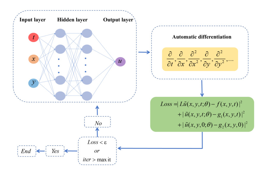
In this paper, an accurate fractional physical information neural network with an adaptive learning rate (adaptive-fPINN-PQI) was first proposed for solving fractional partial differential equations. First, piecewise quadratic interpolation (PQI) in the sense of the Hadamard finite-part integral was introduced in the neural network to discretize the time-fractional derivative in the Caputo sense. Second, the adaptive learning rate residual network was constructed to keep the network from being stuck in the locally optimal solution, which automatically adjusts the weights of different loss terms, significantly balancing their gradients. Additionally, different from the traditional physical information neural networks, this neural network employs a new composite activation function based on the principle of Fourier transform instead of a single activation function, which significantly enhances the network's accuracy. Finally, numerous time-fractional diffusion and time-fractional phase-field equations were solved using the proposed adaptive-fPINN-PQI to demonstrate its high precision and efficiency.
Citation: Ziqing Yang, Ruiping Niu, Miaomiao Chen, Hongen Jia, Shengli Li. Adaptive fractional physical information neural network based on PQI scheme for solving time-fractional partial differential equations[J]. Electronic Research Archive, 2024, 32(4): 2699-2727. doi: 10.3934/era.2024122
In this paper, an accurate fractional physical information neural network with an adaptive learning rate (adaptive-fPINN-PQI) was first proposed for solving fractional partial differential equations. First, piecewise quadratic interpolation (PQI) in the sense of the Hadamard finite-part integral was introduced in the neural network to discretize the time-fractional derivative in the Caputo sense. Second, the adaptive learning rate residual network was constructed to keep the network from being stuck in the locally optimal solution, which automatically adjusts the weights of different loss terms, significantly balancing their gradients. Additionally, different from the traditional physical information neural networks, this neural network employs a new composite activation function based on the principle of Fourier transform instead of a single activation function, which significantly enhances the network's accuracy. Finally, numerous time-fractional diffusion and time-fractional phase-field equations were solved using the proposed adaptive-fPINN-PQI to demonstrate its high precision and efficiency.

| [1] |
Shallu, V. K. Kukreja, An improvised extrapolated collocation algorithm for solving Kuramoto–Sivashinsky equation, Math. Methods Appl. Sci., 45 (2022), 1451–1467. https://doi.org/10.1002/mma.7865 doi: 10.1002/mma.7865

|
| [2] | V. K. Kukreja, An optimal B-spline collocation technique for numerical simulation of viscous coupled Burgers' equation, Comput. Methods Differ. Equations, 10 (2022), 1027–1045. |
| [3] |
Shallu, V. K. Kukreja, An improvised collocation algorithm with specific end conditions for solving modified Burgers equation, Numer. Methods Partial Differ. Equations, 37 (2021), 874–896. https://doi.org/10.1002/num.22557 doi: 10.1002/num.22557
|
| [4] |
F. Y. Song, C. J. Xu, G. E. Karniadakis, A fractional phase-field model for two-phase flows with tunable sharpness: Algorithms and simulations, Comput. Methods Appl. Mech. Eng., 305 (2016), 376–404. https://doi.org/10.1016/i.cma.2016.03.018 doi: 10.1016/i.cma.2016.03.018
|
| [5] |
B. E. Treeby, B. T. Cox, Modeling power law absorption and dispersion for acoustic propagation using the fractional Laplacian, J. Acoust. Soc. Am., 127 (2010), 2741–2748. https://doi.org/10.1121/1.3377056 doi: 10.1121/1.3377056
|
| [6] |
S. Holm, S. P. Nasholm, Comparison of fractional wave equations for power-law attenuation in ultrasound and elastography, Ultrasound. Med. Biol., 40 (2014), 695–703. https://doi.org/10.1016/j.ultrasmedbio.2013.09.033 doi: 10.1016/j.ultrasmedbio.2013.09.033
|
| [7] |
T. Y. Zhu, J. M. Harris, Modeling acoustic wave propagation in heterogeneous attenuating media using decoupled fractional Laplacians, Geophysics, 79 (2014), T105–T116. https://doi.org/10.1190/geo2013-0245.1 doi: 10.1190/geo2013-0245.1
|
| [8] |
W. Zhang, A. Capilnasiu, G. Sommer, G. A. Holzapfel, N. A. Nordsletten, An efficient and accurate method for modeling nonlinear fractional viscoelastic biomaterial, Comput. Methods Appl. Mech. Eng., 2020, 362 (2020), 112834. https://doi.org/10.1016/j.cma.2020.112834 doi: 10.1016/j.cma.2020.112834
|
| [9] |
Q. W. Xu, Y. F. Xu, Quenching study of two-dimensional fractional reaction-diffusion equation from combustion process, Comput. Math. Appl, 78 (2019), 1490–1506. https://doi.org/10.1016/j.camwa.2019.04.006 doi: 10.1016/j.camwa.2019.04.006
|
| [10] | K. A. Mustapha, K. M. Furati, O. M. Knio, O. P. Le Maî tre, A finite difference method for space fractional differential equations with variable diffusivity coefficient, Commun. Appl. Math. Comput., 2 (2020), 671–688. https://link.springer.com/article/10.1007/s42967-020-00066-6 |
| [11] |
A. M. Vargas, Finite difference method for solving fractional differential equations at irregular meshes, Math. Comput., 193 (2022), 204–216. https://doi.org/10.1016/j.matcom.2021.10.010 doi: 10.1016/j.matcom.2021.10.010
|
| [12] | K. Nedaiasl, R. Dehbozorgi, Galerkin finite element method for nonlinear fractional differential equations, Numer. Algorithms, 88 (2021), 113–141. https://link.springer.com/article/10.1007/s11075-020-01032-2 |
| [13] | F. H. Zeng, C. P. Li, F. W. Liu, I. Turner, The use of finite difference/element approaches for solving the time-fractional subdiffusion equation, SIAM J. Sci. Comput., 35 (2013), A2976–A3000. https://epubs.siam.org/doi/10.1137/130910865 |
| [14] | C. L. Wang, Z. Q. Wang, L. L. Wang, A spectral collocation method for nonlinear fractional boundary value problems with a Caputo derivative, J. Sci. Comput., 76 (2018), 166–188. https://link.springer.com/article/10.1007/s10915-017-0616-3 |
| [15] | C. P. Li, F. H. Zeng, F. W. Liu, Spectral approximations to the fractional integral and derivative, Fractional Calculus Appl. Anal., 15 (2012), 383–406. https://link.springer.com/article/10.2478/s13540-012-0028-x |
| [16] |
F. W. Liu, S. Shen, V. Anh, I. Turner, Analysis of a discrete non-markovian random walk approximation for the time fractional diffusion equation, Aust. N. Z. Ind. Appl. Math. J., 46 (2004), C488–C504. https://doi.org/10.21914/anziamj.v46i0.973 doi: 10.21914/anziamj.v46i0.973
|
| [17] |
T. A. M. Langlands, B. I. Henry, The accuracy and stability of an implicit solution method for the fractional diffusion equation, J. Comput. Phys., 205 (2005), 719–736. https://doi.org/10.1016/j.jcp.2004.11.025 doi: 10.1016/j.jcp.2004.11.025
|
| [18] |
Y. Lin, C. Xu, Finite difference/spectral approximations for the time-fractional diffusion equation, J. Comput. Phys., 225 (2007), 1533–1552. https://doi.org/10.1016/j.jcp.2007.02.001 doi: 10.1016/j.jcp.2007.02.001
|
| [19] | W. Deng, Finite element method for the space and time fractional fokker-planck equation, Soc. Ind. Appl. Math., 47 (2008), 204–216. https://epubs.siam.org/doi/abs/10.1137/080714130 |
| [20] | Y. Yan, K. Pal, N. J. Ford, Higher order numerical methods for solving fractional differential equations, BIT Numer. Math., 54 (2014), 555–584. https://link.springer.com/article/10.1007/s10543-013-0443-3 |
| [21] | G. R. Liu, J. Zhang, K. Y. Lam, H. Li, G. Xu, Z. H. Zhong, et al., A gradient smoothing me-thod (GSM) with directional correction for solid mechanics problems, Comput. Mech., 41 (2008), 457–472. https://link.springer.com/article/10.1007/s00466-007-0192-8 |
| [22] |
M. Li, P. H. Wen, Finite block method for transient heat conduction analysis in functionally graded media, Int. J. Numer. Meth. Eng., 99 (2014), 372–390. https://doi.org/10.1002/nme.4693 doi: 10.1002/nme.4693
|
| [23] |
M. Li, Y. C. Hon, T. Korakianitis, P. H. Wen, Finite integration method for nonlocal elastic bar under static and dynamic loads, Eng. Anal. Bound. Elem., 37 (2013), 842–849. https://doi.org/10.1016/j.enganabound.2013.01.018 doi: 10.1016/j.enganabound.2013.01.018
|
| [24] | B. Ahmad, A. Alsaedi, S. K. Ntouyas, J. Tariboon, Hadamard-Type Fractional Differential Equations, Inclusions and Inequalities, Springer International Publishing, 2017. |
| [25] |
M. Li, C. S. Chen, Y. C. Hon, P. H. Wen, Finite integration method for solving multi-dimensional partial differential equations, Appl. Math. Modell., 39 (2015), 4979–4994. https://doi.org/10.1016/j.apm.2015.03.049 doi: 10.1016/j.apm.2015.03.049
|
| [26] |
S. Brunton, J. Proctor, J. Kutz, Discovering governing equations from data by sparse identification of nonlinear dynamical systems, Proc. Nat. Acad. Sci., 113 (2016), 3932–3937. https://doi.org/10.1073/pnas.1517384113 doi: 10.1073/pnas.1517384113
|
| [27] |
S. Brunton, B. Noack, P. Koumoutsakos, Machine learning for fluid mechanics, Annu. Rev. Fluid Mech., 52 (2020), 477–508. https://doi.org/10.1146/annurev-fluid-010719-060214 doi: 10.1146/annurev-fluid-010719-060214
|
| [28] |
W. S. Zha, W. Zhang, D. L. Li, Y. Xing, L. He, J. Q. Tan, Convolution-based model-solving method for three-dimensional, unsteady, partial differential equations, Neural Comput., 34 (2022), 518–540. https://doi.org/10.1016/j.jcp.2019.108925 doi: 10.1016/j.jcp.2019.108925
|
| [29] | Z. C. Long, Y. P. Lu, B. Dong, PDE-Net 2.0: Learning PDEs from data with a numeric-symbolic hybrid deep network, J. Comput. Phys., 399 (2019), 108925. |
| [30] |
R. Zhao, R. Yan, Z. Chen, K. Mao, P. Wang, R. Gao, Deep learning and its applications to machine health monitoring, Mech. Syst. Signal Process, 115 (2019), 213–237. https://doi.org/10.48550/arXiv.1612.07640 doi: 10.48550/arXiv.1612.07640
|
| [31] |
Q. Wang, G. Zhang, C. Sun, N. Wu, High efficient load paths analysis with U index generated by deep learning, Comput. Methods Appl. Mech. Eng., 344 (2019), 499–511. https://doi.org/10.1016/j.cma.2018.10.012 doi: 10.1016/j.cma.2018.10.012
|
| [32] |
D. Finol, Y. Lu, V. Mahadevan, A. Srivastava, Deep convolutional neural networks for eigenvalue problems in mechanics, Int. J. Numer. Methods Eng., 118 (2019), 258–275. https://doi.org/10.48550/arXiv.1801.05733 doi: 10.48550/arXiv.1801.05733
|
| [33] | W. Zheng, F. T. Weng, J. L. Liu, K. Cao, M. Z. Hou, J. Wang, Numerical solution for high dimensional partial differential equations based on deep learning with residual learning and data-driven learning, Int. J. Mach. Learn. Cybern., 12 (2021), 1839–1851. https://link.springer.com/article/10.1007/s13042-021-01277-w |
| [34] |
B. Yohai, S. Hoyer, J. Hickey, M. P. Brenner, Learning data-driven discretizations for partial differential equations, Proceed. Nat. Acad. Sci., 116 (2019), 201814058. https://doi.org/10.1073/pnas.1814058116 doi: 10.1073/pnas.1814058116
|
| [35] |
M. Raissi, P. Perdikaris, G. Karniadakis, Physics-informed neural networks: A deep learning framework for solving forward and inverse problems involving nonlinear partial differential equations, J. Comput. Phys., 378 (2019), 686–707. https://doi.org/10.1016/j.jcp.2018.10.045 doi: 10.1016/j.jcp.2018.10.045
|
| [36] |
E. Kharazmi, Z. Zhang, G. Karniadakis, hp-VPINNs: Variational physics-informed neural networks with domain decomposition, Comput. Methods Appl. Mech. Eng., 374 (2021), 113547. https://doi.org/10.1016/j.cma.2020.113547 doi: 10.1016/j.cma.2020.113547
|
| [37] |
G. Pang, M. D'Elia, M. Parks, M. Karniadakis, nPINNs: Nonlocal physics-informed neural networks for a parametrized nonlocal universal Laplacian operator, Algorithms and applications, J. Comput. Phys., 422 (2020), 109760. https://doi.org/10.1016/j.jcp.2020.109760 doi: 10.1016/j.jcp.2020.109760
|
| [38] |
A. Jagtap, G. Karniadakis, Extended physics-informed neural networks (XPINNs): A generalized space-time domain decomposition based deep learning framework for nonlinear partial differential equations, Commun. Comput. Phys., 28 (2020), 2002–2041. https://doi.org/10.4208/cicp.oa-2020-0164 doi: 10.4208/cicp.oa-2020-0164
|
| [39] |
Q. Zheng, L. Zeng, G. Karniadakis, Physics-informed semantic inpainting: Application to geostatistical modeling, J. Comput. Phys., 419 (2020), 109676. https://doi.org/10.1016/j.jcp.2020.109676 doi: 10.1016/j.jcp.2020.109676
|
| [40] |
L. Yang, X. Meng, G. E. Karniadakis, B-PINNS: Bayesian physics-informed neural networks for forward and inverse PDE problems with noisy data, J. Comput. Phys., 425 (2021), 109913. https://doi.org/10.1016/j.jcp.2020.109913 doi: 10.1016/j.jcp.2020.109913
|
| [41] |
L. Guo, H. Wu, X. Yu, T. Zhou, Monte Carlo PINNS: Deep learning approach for forward and inverse problems involving high dimensional fractional partial differential equations, Comput. Methods Appl. Mech. Eng., 400 (2022), 115523. https://doi.org/10.1016/j.cma.2022.115523 doi: 10.1016/j.cma.2022.115523
|
| [42] |
J. Sirignano, K. Spiliopoulos, DGM: A deep learning algorithm for solving partial differential equations, J. Comput. Phys., 375 (2018), 1339–1364. https://doi.org/10.1016/j.jcp.2018.08.029 doi: 10.1016/j.jcp.2018.08.029
|
| [43] | W. E, B. Yu, The deep Ritz method: A deep learning-based numerical algorithm for solving variational problems, Commun. Math. Stat., 6 (2018), 1–12. https://link.springer.com/article/10.1007/s40304-018-0127-z |
| [44] |
L. Lyu, Z. Zhang, M. Chen, J. Chen, MIM: A deep mixed residual method for solving high-order partial differential equations, J. Comput. Phys., 452 (2022), 110930. https://doi.org/10.1016/j.jcp.2021.110930 doi: 10.1016/j.jcp.2021.110930
|
| [45] |
L. Yang, X. Meng, G. E. Karniadakis, B-PINNS: Bayesian physics-informed neural networks for forward and inverse PDE problems with noisy data, J. Comput. Phys., 425 (2021), 109913. https://doi.org/10.1016/j.jcp.2020.109913 doi: 10.1016/j.jcp.2020.109913
|
| [46] | J. Hou, Y. Li, S. Ying, Enhancing PINNs for solving PDEs via adaptive collocation point movement and adaptive loss weighting, Nonlinear Dyn., 111 (2023), 15233–15261. https://link.springer.com/article/10.1007/s11071-023-08654-w |
| [47] |
S. N. Lin, Y. Chen, A two-stage physics-informed neural network method based on conserved quantities and applications in localized wave solutions, J. Comput. Phys., 457 (2022), 111053. https://doi.org/10.1016/j.jcp.2022.111053 doi: 10.1016/j.jcp.2022.111053
|
| [48] |
J. C. Pu, Y. Chen, Complex dynamics on the one-dimensional quantum droplets via time piecewise PINNs, Phys. D, 454 (2023), 133851. https://doi.org/10.1016/j.physd.2023.133851 doi: 10.1016/j.physd.2023.133851
|
| [49] |
S. N. Lin, Y. Chen, Physics-informed neural network methods based on Miura transformations and discovery of new localized wave solutions, Phys. D, 445 (2023), 133629. https://doi.org/10.1016/j.physd.2022.133629 doi: 10.1016/j.physd.2022.133629
|
| [50] |
J. C. Pu, Y. Chen, Data-driven vector localized waves and parameters discovery for Manakov system using deep learning approach, Chaos Solitons Fractals, 160 (2022), 112182. https://doi.org/10.1016/j.chaos.2022.112182 doi: 10.1016/j.chaos.2022.112182
|
| [51] |
G. Pang, L. Lu, G. Karniadakis, fPINNs: Fractional physics informed neural networks, SIAM J. Sci. Comput, 41 (2019), 2603–2626. https://doi.org/10.1137/18M1229845 doi: 10.1137/18M1229845
|
| [52] |
F. Rostami, A. Jafarian, A new artificial neural network structure for solving high-order linear fractional differential equations, Int. J. Comput. Math., 95 (2018), 528–539. https://doi.org/10.1080/00207160.2017.1291932 doi: 10.1080/00207160.2017.1291932
|
| [53] | S. P. Wang, H. Zhang, X. Jiang, Fractional physics-informed neural networks for time-fractional phase field models, Nonlinear Dyn., 110 (2022), 2715–2739. https://link.springer.com/article/10.1007/s11071-022-07746-3 |
| [54] |
Z. Li, Y. Yan, N. J. Ford, Error estimates of a high order numerical method for solving linear fractional differential equations, Appl. Numer. Math., 114 (2017), 201–220. https://doi.org/10.1016/j.apnum.2016.04.0107 doi: 10.1016/j.apnum.2016.04.0107
|
| [55] | K. Diethelm, An algorithm for the numerical solution of differential equations of fractional order, Electron. Trans. Numer. Anal., 5 (1997), 1–6. |
| [56] | M. Chen, R. Niu, W. Zheng, Adaptive multi-scale neural network with Resnet blocks for solving partial differential equations, Nonlinear Dyn., 111 (2023), 6499–6518. https://link.springer.com/article/10.1007/s11071-022-08161-4 |
| [57] |
Z. Miao, Y. Chen, VC-PINN: Variable coefficient physics-informed neural network for forward and inverse problems of PDEs with variable coefficient, Phys. D, 456 (2023), 133945. https://doi.org/10.1016/j.physd.2023.133945 doi: 10.1016/j.physd.2023.133945
|
| [58] | M. Abu-Shady, M. K. A. Kaabar, A generalized definition of fractional derivative with applications, Math. Probl. Eng., (2021). https://doi.org/10.1155/2021/9444803 |


Figures(19) / Tables(7)
Ziqing Yang, Ruiping Niu, Miaomiao Chen, Hongen Jia, Shengli Li. Adaptive fractional physical information neural network based on PQI scheme for solving time-fractional partial differential equations[J]. Electronic Research Archive, 2024, 32(4): 2699-2727. doi: 10.3934/era.2024122


 DownLoad: