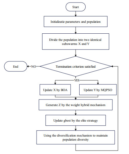
This paper presents a novel hybrid algorithm that combines the Butterfly Optimization Algorithm (BOA) and Quantum-behavior Particle Swarm Optimization (QPSO) algorithms, leveraging $ gbest $ to establish an algorithm communication channel for cooperation. Initially, the population is split into two equal subgroups optimized by BOA and QPSO respectively, with the latter incorporating the Lévy flight for enhanced performance. Subsequently, a hybrid mechanism comprising a weight hybrid mechanism, a elite strategy, and a diversification mechanism is introduced to blend the two algorithms. Experimental evaluation on 12 benchmark test functions and the Muskin model demonstrates that the synergy between BOA and QPSO significantly enhances algorithm performance. The hybrid mechanism further boosts algorithm performance, positioning the new algorithm as a high-performance method. In the Muskingum model experiment, the algorithm proposed in this article can give the best sum of the square of deviation (SSQ) and is superior in the comparison of other indicators. Overall, through benchmark test function experiments and Muskin model evaluations, it is evident that the algorithm proposed in this paper exhibits strong optimization capabilities and is effective in addressing practical problems.
Citation: Hanbin Liu, Libin Liu, Xiongfa Mai, Delong Guo. A new hybrid Lévy Quantum-behavior Butterfly Optimization Algorithm and its application in NL5 Muskingum model[J]. Electronic Research Archive, 2024, 32(4): 2380-2406. doi: 10.3934/era.2024109
This paper presents a novel hybrid algorithm that combines the Butterfly Optimization Algorithm (BOA) and Quantum-behavior Particle Swarm Optimization (QPSO) algorithms, leveraging $ gbest $ to establish an algorithm communication channel for cooperation. Initially, the population is split into two equal subgroups optimized by BOA and QPSO respectively, with the latter incorporating the Lévy flight for enhanced performance. Subsequently, a hybrid mechanism comprising a weight hybrid mechanism, a elite strategy, and a diversification mechanism is introduced to blend the two algorithms. Experimental evaluation on 12 benchmark test functions and the Muskin model demonstrates that the synergy between BOA and QPSO significantly enhances algorithm performance. The hybrid mechanism further boosts algorithm performance, positioning the new algorithm as a high-performance method. In the Muskingum model experiment, the algorithm proposed in this article can give the best sum of the square of deviation (SSQ) and is superior in the comparison of other indicators. Overall, through benchmark test function experiments and Muskin model evaluations, it is evident that the algorithm proposed in this paper exhibits strong optimization capabilities and is effective in addressing practical problems.

| [1] |
A. Ouyang, Y. Lu, Y. Liu, M. Wu, X. Peng, An improved adaptive genetic algorithm based on DV-Hop for locating nodes in wireless sensor networks, Neurocomputing, 458 (2021), 500–510. https://doi.org/10.1016/j.neucom.2020.04.156 doi: 10.1016/j.neucom.2020.04.156

|
| [2] |
J. Lin, S. X. Zhang, S. Y. Zheng, Y. M. Pan, Differential evolution with fusion of local and global search strategies, J. Comput. Sci., 63 (2022), 101746. https://doi.org/10.1016/j.jocs.2022.101746 doi: 10.1016/j.jocs.2022.101746
|
| [3] |
W. He, B. Wang, N. Li, X. Gao, W. Li, Q. Jiang, An improved Sine-Cosine algorithm with dynamic selection pressure, J. Comput. Sci., 55 (2021), 101477. https://doi.org/10.1016/j.jocs.2021.101477 doi: 10.1016/j.jocs.2021.101477
|
| [4] |
D. Simon, Biogeography-based optimization, IEEE Trans. Evol. Comput., 12 (2008), 702–713. https://doi.org/10.1109/TEVC.2008.919004 doi: 10.1109/TEVC.2008.919004
|
| [5] |
S. Khan, M. Kamran, O. U. Rehman, L. Liu, S. Yang, A modified PSO algorithm with dynamic parameters for solving complex engineering design problem, Int. J. Comput. Math., 95 (2018), 2308–2329. https://doi.org/10.1080/00207160.2017.1387252 doi: 10.1080/00207160.2017.1387252
|
| [6] |
S. Mitra, S. Acharyya, Perturbation and repository based diversified cuckoo search in reconstruction of gene regulatory network: A new cuckoo search approach, J. Comput. Sci., 60 (2022), 101600. https://doi.org/10.1016/j.jocs.2022.101600 doi: 10.1016/j.jocs.2022.101600
|
| [7] |
S. Arora, S. Singh, Butterfly optimization algorithm: a novel approach for global optimization, Soft Comput., 23 (2019), 715–734. https://doi.org/10.1007/s00500-018-3102-4 doi: 10.1007/s00500-018-3102-4
|
| [8] |
D. H. Wolpert, W. G. Macready, No free lunch theorems for optimization, IEEE Trans. Evol. Comput., 1 (1997), 67–82. https://doi.org/10.1109/4235.585893 doi: 10.1109/4235.585893
|
| [9] |
C. Zhong, G. Li, Z. Meng, W. He, Opposition-based learning equilibrium optimizer with Levy flight and evolutionary population dynamics for high-dimensional global optimization problems, Expert Syst. Appl., 215 (2023), 119303. https://doi.org/10.1016/j.eswa.2022.119303 doi: 10.1016/j.eswa.2022.119303
|
| [10] |
G. Tian, Y. Ren, Y. Feng, M. Zhou, H. Zhang, J. Tan, Modeling and planning for dual-objective selective disassembly using AND/OR graph and discrete artificial bee colony, IEEE Trans. Ind. Inf., 15 (2018), 2456–2468. https://doi.org/10.1109/TII.2018.2884845 doi: 10.1109/TII.2018.2884845
|
| [11] |
S. Lou, Y. Zhang, R. Tan, C. Lv, A smooth path planning method for mobile robot using a BES-incorporated modified QPSO algorithm, Expert Syst. Appl., 208 (2022), 118256. https://doi.org/10.1016/j.eswa.2022.118256 doi: 10.1016/j.eswa.2022.118256
|
| [12] |
S. Dian, J. Zhong, B. Guo, J. Liu, R. Guo, A human-cyber-physical system enabled sequential disassembly planning approach for a human-robot collaboration cell in Industry 5.0, Rob. Comput. Integr. Manuf., 208 (2022), 118256. https://doi.org/10.1016/j.rcim.2023.102706 doi: 10.1016/j.rcim.2023.102706
|
| [13] |
K. Aygül, M. Cikan, T. Demirdelen, M. Tumay, Butterfly optimization algorithm based maximum power point tracking of photovoltaic systems under partial shading condition, Energy Sources Part A, 45 (2023), 8337–8355. https://doi.org/10.1080/15567036.2019.1677818 doi: 10.1080/15567036.2019.1677818
|
| [14] |
S. Arora, P. Anand, Learning automata-based butterfly optimization algorithm for engineering design problems, Int. J. Comput. Mater. Sci. Eng., 7 (2018), 1850021. https://doi.org/10.1142/S2047684118500215 doi: 10.1142/S2047684118500215
|
| [15] |
G. Li, F. Shuang, P. Zhao, C. Le, An improved butterfly optimization algorithm for engineering design problems using the cross-entropy method, Symmetry, 11 (2019), 1049. https://doi.org/10.3390/sym11081049 doi: 10.3390/sym11081049
|
| [16] |
Y. Fan, J. Shao, G. Sun, X. Shao, A self-adaption butterfly optimization algorithm for numerical optimization problems, IEEE Access, 2021 (2021), 88026–88041. https://doi.org/10.1109/ACCESS.2020.2993148 doi: 10.1109/ACCESS.2020.2993148
|
| [17] |
Y. Li, X. Yu, J. Liu, Enhanced butterfly optimization algorithm for large-scale optimization problems, J. Bionic. Eng., 19 (2022), 554–570. https://doi.org/10.1007/s42235-021-00143-3 doi: 10.1007/s42235-021-00143-3
|
| [18] |
A. Assiri, On the performance improvement of butterfly optimization approaches for global optimization and feature selection, PLoS One, 16 (2021), 0242612. https://doi.org/10.1371/journal.pone.0242612 doi: 10.1371/journal.pone.0242612
|
| [19] |
M. W. Li, D. Y. Xu, J. Geng, W. C. Hong, A ship motion forecasting approach based on empirical mode decomposition method hybrid deep learning network and quantum butterfly optimization algorithm, Nonlinear Dyn., 107 (2022), 2447–2467. https://doi.org/10.1007/s11071-021-07139-y doi: 10.1007/s11071-021-07139-y
|
| [20] |
Z. Wang, Q. Luo, Y. Zhou, Hybrid metaheuristic algorithm using butterfly and flower pollination base on mutualism mechanism for global optimization problems, Eng. Comput., 37 (2020), 3665–3698. https://doi.org/10.1007/S00366-020-01025-8 doi: 10.1007/S00366-020-01025-8
|
| [21] |
A. Toktas, D. Ustun, A triple-objective optimization scheme using butterfly integrated ABC algorithm for design of multilayer RAM, IEEE Trans. Antennas Propag., 68 (2020), 5602–5612. https://doi.org/10.1109/TAP.2020.2981728 doi: 10.1109/TAP.2020.2981728
|
| [22] |
Z. A. Dahi, C. Mezioud, A. Draa, A quantum-inspired genetic algorithm for solving the antenna positioning problem, Swarm Evol. Comput., 31 (2016), 24–36. https://doi.org/10.1016/j.swevo.2016.06.003 doi: 10.1016/j.swevo.2016.06.003
|
| [23] |
S. Dey, S. Bhattacharyya, U. Maulik, Quantum inspired genetic algorithm and particle swarm optimization using chaotic map model based interference for gray level image thresholding, Swarm Evol. Comput., 15 (2014), 38–57. https://doi.org/10.1016/j.swevo.2013.11.002 doi: 10.1016/j.swevo.2013.11.002
|
| [24] |
B. Liu, Y. Zhou, Q. Luo, H. Huang, Quantum-inspired African vultures optimization algorithm with elite mutation strategy for production scheduling problems, J. Comput. Des. Eng., 10 (2023), 1767–1789. https://doi.org/10.1093/jcde/qwad078 doi: 10.1093/jcde/qwad078
|
| [25] |
R. N. D. Costa-Filho, Comparative study of three quantum-inspired optimization algorithms for robust tuning of power system stabilizers, Neural Comput. Appl., 35 (2023), 12905–12914. https://doi.org/10.1007/s00521-023-08429-9 doi: 10.1007/s00521-023-08429-9
|
| [26] | J. Sun, B. Feng, W. Xu, Particle swarm optimization with particles having quantum behavior, in Proceedings of the 2004 Congress on Evolutionary Computation, Portland, OR, USA, (2004), 111–116. |
| [27] |
N. Kumar, A. A. Shaikh, S. K. Mahato, A. K. Bhunia, Applications of new hybrid algorithm based on advanced cuckoo search and adaptive Gaussian quantum behaved particle swarm optimization in solving ordinary differential equations, Expert Syst. Appl., 172 (2021), 114646. https://doi.org/10.1016/j.eswa.2021.114646 doi: 10.1016/j.eswa.2021.114646
|
| [28] |
X. Mai, H. B. Liu, L. B. Liu, A new hybrid cuckoo quantum-behavior particle swarm optimization algorithm and its application in Muskingum model, Neural Process. Lett., 55 (2023), 8309–8337. https://doi.org/10.1007/s11063-023-11313-1 doi: 10.1007/s11063-023-11313-1
|
| [29] |
C. Wang, Z. Wang, S. Zhang, J. Tan, Adam-assisted quantum particle swarm optimization guided by length of potential well for numerical function optimization, Swarm Evol. Comput., 79 (2023), 101309. https://doi.org/10.1016/j.swevo.2023.101309 doi: 10.1016/j.swevo.2023.101309
|
| [30] |
Y. Ling, Y. Zhou, Q. Luo, Lévy flight trajectory-based whale optimization algorithm for global optimization, IEEE Access, 5 (2017), 6168–6186. https://doi.org/10.1109/ACCESS.2017.2695498 doi: 10.1109/ACCESS.2017.2695498
|
| [31] |
C. Zhong, G. Li, Z. Meng, W. He, Opposition-based learning equilibrium optimizer with Levy flight and evolutionary population dynamics for high-dimensional global optimization problems, Expert Syst. Appl., 15 (2023), 119303. https://doi.org/10.1016/j.eswa.2022.1193032 doi: 10.1016/j.eswa.2022.1193032
|
| [32] |
R. Sihwail, K. Omar, K. A. Z. Ariffin, M. Tubishat, Improved Harris Hawks optimization using elite opposition-based learning and novel search mechanism for feature selection, IEEE Access, 8 (2020), 121127–121145. https://doi.org/10.1109/ACCESS.2020.3006473 doi: 10.1109/ACCESS.2020.3006473
|
| [33] |
M. A. Elaziz, D. Yousri, S. Mirjalili, A hybrid Harris hawks-moth-flame optimization algorithm including fractional-order chaos maps and evolutionary population dynamics, Adv. Eng. Software, 154 (2021), 102973. https://doi.org/10.1016/j.advengsoft.2021.102973 doi: 10.1016/j.advengsoft.2021.102973
|
| [34] |
W. C. Wang, W. C. Tian, D. M. Xu, K. W. Chau, Q. Ma, C. J. Liu, Muskingum models' development and their parameter estimation: A state-of-the-art review, Water Resour. Manage., 37 (2023), 3129–3150. https://doi.org/10.1007/s11269-023-03493-1 doi: 10.1007/s11269-023-03493-1
|
| [35] |
A. Ouyang, L. B. Liu, Z. Sheng, F. Wu, A class of parameter estimation methods for nonlinear Muskingum model using hybrid invasive weed optimization algorithm, Math. Probl. Eng., 2015 (2015), 573894. https://doi.org/10.1155/2015/573894 doi: 10.1155/2015/573894
|
| [36] |
U. Okkan, U. Kirdemir, Locally tuned hybridized particle swarm optimization for the calibration of the nonlinear Muskingum flood routing model, J. Water Clim. Change, 11 (2020), 343–358. https://doi.org/10.2166/wcc.2020.015 doi: 10.2166/wcc.2020.015
|
| [37] |
R. Akbari, M. R. Hessami-Kermani, A new method for dividing food period in the variable-parameter Muskingum models, Hydrol. Res., 53 (2015), 241–257. https://doi.org/10.2166/nh.2021.192 doi: 10.2166/nh.2021.192
|
| [38] | O. B. Haddad, F. Hamedi, M. Orouji, M. Pazoko, H. A. Loáiciga, A re-parameterized and improved nonlinear Muskingum model for flood routing. Water Resour. Manage, 29 (2015), 3419–3440. https://doi.org/10.1007/s11269-015-1008-9 |
| [39] |
X. Lu, G. He, QPSO algorithm based on Levy flight and its application in fuzzy portfolio, Appl. Soft Comput., 99 (2020), 106894. https://doi.org/10.1016/j.asoc.2020.106894 doi: 10.1016/j.asoc.2020.106894
|
| [40] |
J. P. Jacob, K. Pradeep, A multi-objective optimal task scheduling in cloud environment using cuckoo particle swarm optimization, Wireless Pers. Commun., 109 (2019), 315–331. https://doi.org/10.1007/s11277-019-06566-w doi: 10.1007/s11277-019-06566-w
|
| [41] | B. Wang, J. Wei, Particle swarm optimization with genetic evolution for task offloading in device-edge-cloud collaborative computing, in Advanced Intelligent Computing Technology and Applications. ICIC 2023 (eds. D. S. Huang, P. Premaratne, B. Jin, B. Qu, K. H. Jo, A. Hussain), Springer Nature Singapore, (2023), 340–350. https://doi.org/10.1007/978-981-99-4761-4_29 |
| [42] |
S. Wang, Y. Li, H. Yang, Self-adaptive mutation differential evolution algorithm based on particle swarm optimization, Appl. Soft Comput., 81 (2019), 105496. https://doi.org/10.1016/j.asoc.2019.105496 doi: 10.1016/j.asoc.2019.105496
|
| [43] |
Z. Yu, J. Du, Constrained fault-tolerant thrust allocation of ship DP system based on a novel quantum-behaved squirrel search algorithm, Ocean Eng., 266 (2022), 112994. https://doi.org/10.1016/j.oceaneng.2022.112994 doi: 10.1016/j.oceaneng.2022.112994
|
| [44] |
F. A. Hashim, E. H. Houssein, K. Hussain, M. S. Mabrouk, W. Al-Atabany, Honey badger algorithm: New metaheuristic algorithm for solving optimization problems, Math. Comput. Simul., 192 (2022), 84–110. https://doi.org/10.1016/j.matcom.2021.08.013 doi: 10.1016/j.matcom.2021.08.013
|
| [45] |
A. Faramarzi, M. Heidarinejad, S. Mirjalili, A. H. Gandomi, Marine predators algorithm: A nature-inspired metaheuristic, Expert Syst. Appl., 152 (2020), 113377. https://doi.org/10.1016/j.eswa.2020.113377 doi: 10.1016/j.eswa.2020.113377
|
| [46] |
Y. Xia, Z. Feng, W. Niu, H. Qin, Z. Jiang, J. Zhou, Simplex quantum-behaved particle swarm optimization algorithm with application to ecological operation of cascade hydropower reservoirs, Appl. Soft Comput., 84 (2019), 105715. https://doi.org/10.1016/j.asoc.2019.105715 doi: 10.1016/j.asoc.2019.105715
|
| [47] | E. M. Wilson, Engineering hydrology, MacMillan Education, London, 1974. |
| [48] |
S. M. Easa, Improved nonlinear Muskingum model with variable exponent parameter, J. Hydrol. Eng., 18 (2013), 1790–1794. https://doi.org/10.1061/(ASCE)HE.1943-5584.0000702 doi: 10.1061/(ASCE)HE.1943-5584.0000702
|
| [49] | W. Viessman, G. Lewis, Introduction to Hydrology, Archaea, the United State, 2003. |


Figures(8) / Tables(13)
Hanbin Liu, Libin Liu, Xiongfa Mai, Delong Guo. A new hybrid Lévy Quantum-behavior Butterfly Optimization Algorithm and its application in NL5 Muskingum model[J]. Electronic Research Archive, 2024, 32(4): 2380-2406. doi: 10.3934/era.2024109


 DownLoad: