Estimation of spatiotemporal travel speed based on probe vehicles in mixed traffic flow

Jongho Kim; Woosuk Kim; Eunjeong Ko; Yong-Shin Kang; Hyungjoo Kim; Jongho Kim; Woosuk Kim; Eunjeong Ko; Yong-Shin Kang; Hyungjoo Kim

doi:10.3934/era.2024015

Electronic Research Archive

2024, Volume 32, Issue 1: 317-331. doi: 10.3934/era.2024015

Previous Article Next Article

Research article Special Issues

Estimation of spatiotemporal travel speed based on probe vehicles in mixed traffic flow

1.
Cho Chun Shik Graduate School of Mobility, Korea Advanced Institute of Science and Technology CCS Graduate School of Mobility, Yuseonggu, Daejeon 193, Republic of Korea
2.
Department of Intelligent Transportation System Lab, Advanced Institute of Convergence Technology, Suwon-si, Gyeonggi-do 16229, Republic of Korea
3.
Industrial Intelligence Laboratory, Advanced Institute of Convergence Technology, Suwon-si, Gyeonggi-do 16229, Republic of Korea

Received: 20 October 2023 Revised: 21 November 2023 Accepted: 03 December 2023 Published: 25 December 2023

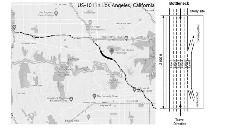
Conventional fixed traffic detectors are limited to their installed locations and are unable to collect general traffic information or monitor microscopic traffic flows. Mobile detectors overcome spatial constraints by allowing the vehicle to act as a detector and can observe microscopic traffic flows by collecting high-resolution trajectory data from individual vehicles. The objective of this study is to estimate spatiotemporal traffic information based on the autonomous driving sensor headway distance and to calculate the appropriate spatiotemporal interval according to the sampling rate. First, individual vehicle trajectory data was collected, and a traffic information estimation was established. Travel speed was calculated based on generalized definitions, and its estimation and errors were analyzed. In addition, the appropriate spatiotemporal interval according to cell size, time interval, and sampling rate was analyzed. The analysis demonstrated that the estimation accuracy was improved by cell size, time interval, and sampling rate. Based on this, the appropriate time and space to minimize the error rate were calculated considering the sampling rate. When the sampling rate was 40% or more, the error rate was 5% or less in all time and space; however, error rate differences occurred in several cases at sampling rates below 40%. These results are anticipated for efficient management of collecting, processing and providing traffic information.
- spatiotemporal travel speed,
- probe vehicle,
- NGSIM,
- mixed traffic flow
Citation: Jongho Kim, Woosuk Kim, Eunjeong Ko, Yong-Shin Kang, Hyungjoo Kim. Estimation of spatiotemporal travel speed based on probe vehicles in mixed traffic flow[J]. Electronic Research Archive, 2024, 32(1): 317-331. doi: 10.3934/era.2024015

Related Papers:

Abstract

Conventional fixed traffic detectors are limited to their installed locations and are unable to collect general traffic information or monitor microscopic traffic flows. Mobile detectors overcome spatial constraints by allowing the vehicle to act as a detector and can observe microscopic traffic flows by collecting high-resolution trajectory data from individual vehicles. The objective of this study is to estimate spatiotemporal traffic information based on the autonomous driving sensor headway distance and to calculate the appropriate spatiotemporal interval according to the sampling rate. First, individual vehicle trajectory data was collected, and a traffic information estimation was established. Travel speed was calculated based on generalized definitions, and its estimation and errors were analyzed. In addition, the appropriate spatiotemporal interval according to cell size, time interval, and sampling rate was analyzed. The analysis demonstrated that the estimation accuracy was improved by cell size, time interval, and sampling rate. Based on this, the appropriate time and space to minimize the error rate were calculated considering the sampling rate. When the sampling rate was 40% or more, the error rate was 5% or less in all time and space; however, error rate differences occurred in several cases at sampling rates below 40%. These results are anticipated for efficient management of collecting, processing and providing traffic information.

References

[1]	H. Kim, Y. Kim, K. Jang, Systematic relation of estimated travel speed and actual travel speed, IEEE Trans. Intell. Transp. Syst., 18 (2017), 2780–2789. https://doi.org/10.1109/tits.2017.2713983 doi: 10.1109/tits.2017.2713983
[2]	G. Kloot, Melbourne's arterial travel time system, in International Conference of Australia, 4th, Adelaide, South Australia, 1999.
[3]	R. J. Haseman, J. S. Wasson, D. M. Bullock, Real-time measurement of travel time delay in work zones and evaluation metrics using Bluetooth probe tracking, Transp. Res. Rec., 2169 (2010), 40–53. https://doi.org/10.3141/2169-05 doi: 10.3141/2169-05
[4]	S. Gao, I. Chabini, Optimal routing policy problems in stochastic time-dependent networks, Transp. Res. Part B Methodol., 40 (2006), 93–122. https://doi.org/10.1016/j.trb.2005.02.001 doi: 10.1016/j.trb.2005.02.001
[5]	D. D. Puckett, M. J. Vickich, Bluetooth-based travel time speed measuring systems development, No. UTCM 09-00-17, Texas Transportation Institute, University Transportation Center for Mobility, 2010.
[6]	A. Haghani, M. Hamedi, K. F. Sadabadi, S. Young, P. Tarnoff, Data collection of freeway travel time ground truth with Bluetooth sensors, Transp. Res. Rec. J. Transp. Res. Board, 2160 (2010), 60–68. https://doi.org/10.3141/2160-07 doi: 10.3141/2160-07
[7]	S. Carrese, E. Cipriani, U. Crisalli, A. Gemma, L. Mannini, Bluetooth traffic data for urban travel time forecast, Transp. Res. Procedia, 52 (2021), 236–243. https://doi.org/10.1016/j.trpro.2021.01.027 doi: 10.1016/j.trpro.2021.01.027
[8]	M. G. Wing, A. Eklund, L. D. Kellogg, Consumer-grade global positioning system (GPS) accuracy and reliability, J. For., 103 (2005), 169–173. https://doi.org/10.1093/jof/103.4.169 doi: 10.1093/jof/103.4.169
[9]	J. Du, M. J. Barth, Next-generation automated vehicle location systems: Positioning at the lane level, IEEE Trans. Intell. Transp. Syst., 9 (2008), 48–57. https://doi.org/10.1109/tits.2007.908141 doi: 10.1109/tits.2007.908141
[10]	Z. Peng, S. Hussain, M. I. Hayee, M. Donath, Acquisition of relative trajectories of surrounding vehicles using GPS and SRC based V2V communication with lane level resolution, in Proceedings of 3rd International Conference on Vehicle Technology and Intelligent Transport Systems, (2017), 242–251. https://doi.org/10.5220/0006304202420251
[11]	Y. S. Li, W. B. Zhang, X. W. Ji, C. X. Ren, J. Wu, Research on lane a compensation method based on multi-sensor fusion, Sensors, 19 (2019), 1584. https://doi.org/10.3390/s19071584 doi: 10.3390/s19071584
[12]	J. M. Kang, T. S. Yoon, E. Kim, J. B. Park, Lane-level map-matching method for vehicle localization using GPS and camera on a high-definition map, Sensors, 20 (2020), 2166. https://doi.org/10.3390/s20082166. doi: 10.3390/s20082166
[13]	J. Kim, D. Lim, Y. Seo, J. J. So, H. Kim, Influence of dedicated lanes for connected and automated vehicles on highway traffic flow, IET Intell. Transp. Syst., 17 (2022), 678–690. https://doi.org/10.1049/itr2.12295 doi: 10.1049/itr2.12295
[14]	H. P. Yu, S. H. Tak, M. J. Park, H. S. Yeo, Impact of autonomous-vehicle-only lanes in mixed traffic conditions, J. Transp. Res. Board, Transp. Res. Rec., 2673 (2019), 430–439. https://doi.org/10.1177/0361198119847475 doi: 10.1177/0361198119847475
[15]	S. L. Lee, C. Oh, S. M. Hong, Exploring lane change safety issues for manually driven vehicles in vehicle platooning environments, IET Intell. Transp. Syst., 12 (2018), 1142–1147. https://doi.org/10.1049/iet-its.2018.5167. doi: 10.1049/iet-its.2018.5167
[16]	J. C. Herrera, D. B. Work, R. Herring, X. J. Ban, Q. Jacobson, A. M. Bayen, Evaluation of traffic data obtained via GPS-enabled mobile phones: The Mobile Century field experiment, Transp. Res. Part C Emerg. Technol., 18 (2010), 568–583. https://doi.org/10.1016/j.trc.2009.10.006 doi: 10.1016/j.trc.2009.10.006
[17]	X. Kong, W. Zhou, G. Shen, W. Zhang, N. Liu, Y. Yang, Dynamic graph convolutional recurrent imputation network for spatiotemporal traffic missing data, Knowl.-Based Syst., 261 (2023), 110188. https://doi.org/10.1016/j.knosys.2022.110188 doi: 10.1016/j.knosys.2022.110188
[18]	S. He, X. Guo, F. Ding, Y. Qi, T. Chen, Freeway traffic speed estimation of mixed traffic using data from connected and autonomous vehicles with a low penetration rate, J. Adv. Transp., 2020 (2020), 1–13. https://doi.org/10.1155/2020/1361583 doi: 10.1155/2020/1361583
[19]	A. Elfar, C. Xavier, A. Talebpour, H. S. Mahmassani, Trafﬁc shockwave detection in a connected environment using the speed distribution of individual vehicles, Transp. Res. Rec.: J. Transp. Res. Board, 2672 (2018), 203–214. https://doi.org/10.1177/0361198118794717 doi: 10.1177/0361198118794717
[20]	W. Ma, S. Qian, High-resolution traffic sensing with probe autonomous vehicles: a data-driven approach, Sensors, 21 (2021), 464. https://doi.org/10.3390/s2 1020464 doi: 10.3390/s21020464
[21]	D. Lim, Y. Seo, E. Ko, J. So, H. Kim, Spatiotemporal traffic density estimation based on ADAS probe data, J. Adv. Transp., 2022 (2022), 5929725. https://doi.org/10.1155/2022/5929725 doi: 10.1155/2022/5929725
[22]	H. K. Kim, Y. Chung, M. Kim, Effect of enhanced ADAS camera capability on traffic state estimation, Sensors, 21 (2021), 1996. https://doi.org/10.3390/s21061996 doi: 10.3390/s21061996
[23]	Z. He, Y. Lv, L. Lu, W. Guan, Constructing spatiotemporal speed contour diagrams: using rectangular or non-rectangular parallelogram cells?, Transp. B Transp. Dyn., 7 (2017), 44–60. https://doi.org/10.1080/21680566.2017.1320774 doi: 10.1080/21680566.2017.1320774
[24]	H. Yao, Q. Li, X. Li, A study of relationships in traffic oscillation features based on field experiments, Transp. Res. Part A Policy Pract., 141 (2020), 339–355. https://doi.org/10.1016/j.tra.2020.09.006 doi: 10.1016/j.tra.2020.09.006
[25]	R. L. Bertini, T. L. Monica, Empirical study of traffic features at a freeway lane drop, J. Transp. Eng., 131 (2005), 397–407. https://doi.org/10.1061/(asce)0733-947x(2005)131:6(397) doi: 10.1061/(asce)0733-947x(2005)131:6(397)
[26]	J. A. Laval, L. Leclercq, A mechanism to describe the formation and propagation of stop-and-go waves in congested freeway traffic, Phil. Trans. R. Soc. A, 368 (2010), 4519–4541. https://doi.org/10.1098/rsta.2010.0138 doi: 10.1098/rsta.2010.0138
[27]	Z. He. L. Zheng, W. Guan, A simple nonparametric-following model driven by field data, Transp. Res. Part B Methodol., 80 (2015), 185–201. https://doi.org/10.1016/j.trb.2015.07.010 doi: 10.1016/j.trb.2015.07.010
[28]	T. Seo, T. Kusakabe, Y. Asakura, Estimation of flow and density using probe vehicles with spacing measurement equipment, Transp. Res. Part C Emerg. Technol., 53 (2015), 134–150. https://doi.org/10.1016/j.trc.2015.01.033 doi: 10.1016/j.trc.2015.01.033
[29]	L. C. Edie, Discussion of Traffic Stream Measurements and Definitions, New York: Port of New York Authority, 1963

Reader Comments

Your name:*

Email:*
© 2024 the Author(s), licensee AIMS Press. This is an open access article distributed under the terms of the Creative Commons Attribution License (http://creativecommons.org/licenses/by/4.0)