Reliability analysis and recovery measure of an urban water network

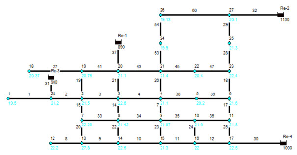
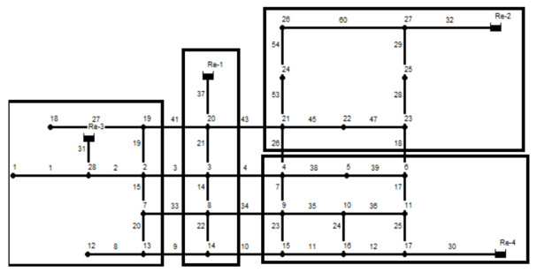
1.   Introduction

The urban water network is an important infrastructure for cities ^[1]. The urban water network guarantees water for urban residents and firefighters through a complex network system ^[2]. However, the urban water network has a complex network topology and a complicated working environment, so it is vulnerable to natural disasters. Furthermore, the urban water network consists of many pipes and valves, so the network is prone to water leakage ^[3]. According to global statistics, at least two-thirds of the world's population experiences large-scale water outages for more than thirty days per year ^[4]. Therefore, the study of the causes of urban water network failure and the response after an accident is crucial to safeguard water for residents and firefighters, which is our concern of this paper.

The occurrence of natural disasters is stochastic, and many scholars have made predictions about the arrival of disasters. A method of describing the arrival time of disasters by Poisson distribution was proposed by ^[5]. Moreover, a part of scholars analyzed the recovery process after the disaster. Song et al. ^[6] proposed a method to determine the optimal recovery sequence of pipelines by considering hydraulic analysis of water networks, pipeline damage and seismic intensity.

The studies of the above scholars have examined the urban water network in detail from the prediction before the arrival of disasters, and with the recovery after the arrival of disasters. Although the above studies are already very comprehensive, there are still some shortcomings. The urban water network is the lifeblood of a city and is the foundation for its smooth operation. In the 1995 earthquake in Kobe, Japan, the maintenance of the urban water network lasted for a month ^[6]. If the ability of the urban water network to resist disasters can be assessed before the earthquake, it will be very favorable to enhance the security of the urban water network. The ability of urban water network to resist disasters refers to the entire cycle before and after the arrival of disasters in the water network. Therefore, rationally analyzing the impact of the disaster on the urban water network and the recovery of the network after the disaster is the key to assessing the ability of the network to resist the disaster.

After a natural disaster, the nodes and edges of the urban water supply network will be affected, and some nodes or edges in the network will fail. The essence of the reliability of an urban water network is to analyze the reliability of a complex network. In the study of the reliability of urban transportation networks, Gu et al. ^[7] systematically reviewed the reliability model of urban transportation network and provided the idea of studying the reliability of urban transportation networks. Gnecco et al. ^[8] proposed a node failure model considering the heterogeneity of nodes. Dui et al. ^[9] studied the network cascading failure under load variation and proposed a maintenance scheme based on the importance of node maintenance priority. Guo et al. ^[10] proposed a cascading failure model for urban transportation networks considering node loads and capacities and provided a detailed analysis of system reliability. Yang et al. ^[11] provided a comprehensive modeling of urban networks and provided a network modeling methodology. Dui et al. ^[12] studied the cascading failure process caused by node or edge failure in a network and performed a collaborative optimization process considering edges and nodes. Zhou et al. ^[13] proposed a model for evaluating network reliability under multiple failure modes considering dependencies. A network reliability calculation method considering entropy was proposed in ^[14]. Xing et al. ^[15] proposed a network node traffic analysis method to analyze network reliability. Shuang et al. ^[16] studied the vulnerability of urban water network nodes under cascading failure. Dui et al. ^[17] investigated the reliability of infrastructure systems under cascading failures in an epidemic situation. Zhang et al. ^[18] proposed a cascading failure method for complex networks with adjustable node load parameters and used different attack methods on the nodes. Wang et al. ^[19] proposed a dynamic cascading failure analysis method for load redistribution. Phan et al. ^[20] established a connectivity-based repair scheme for improving the reliability of water networks after failures. Li et al. ^[21] proposed a network reliability analysis method considering node strength as well as node heterogeneity. Chang et al. ^[22] systematically analyzed the reliability change under the whole process of urban water networks. Many articles have proposed analytical methods for the reliability of the network from different perspectives. These measures, then, are not necessarily suitable for the current reliability study of urban water networks. The purpose of an urban water network is to ensure the water supply for the residents in the city, so the reliability analysis of the urban water network should be analyzed by the indicators related to water supply. Considering the connectivity of the network and the heterogeneity of the nodes obviously cannot meet such requirements. At the same time, the water pressure in the urban water network will also have an impact on the residents' water use. Then, in the above study, the flow rate and water pressure of the nodes are not considered for reliability modeling. Therefore, this paper establishes the reliability modeling of urban water networks from nodes and water pressure.

Many scholars have studied the recovery process of urban water networks after disasters. Li et al. ^[23] detailed the recovery process of the network by analyzing the contribution of the node's already utility. Liu et al. ^[24] proposed two different restoration strategies to repair the network after a disaster. Patriarca et al. ^[25] proposed a technique based on digital twins to identify the critical nodes from the physical system of the network. By analyzing the critical nodes, the repair sequence of the network is determined. Meng et al. ^[26] conducted a comprehensive study on the reliability degradation as well as recovery of water networks including connectivity, efficiency and centrality. Tornyeviadzi et al. ^[27] utilized an integrated AHP-TOPSIS framework to assess the vulnerability of nodes throughout the water network in order to propose the network's optimal recovery strategy. Ebrahimi et al. ^[28] used hydraulic analysis to calculate the reliability of the water network and proposed an optimization strategy. Zarghami et al. ^[29] proposed a methodology to analyze the redundancy of the network by using a coproduction tree as well as information entropy, which provides a specific analysis of the recovery phase of the water network. Liu et al. ^[30] proposed a recovery ratio model considering the minimum reliability constraints of the system. Although many articles have done extensive research on the recovery strategies of urban water networks, the recovery of water networks has not been analyzed in the context of the unpredictability of the occurrence of disasters. In this paper, the recovery process of urban water networks is analyzed in terms of the network state after a disaster.

In this paper, the work carried out is compared with other literature as shown in Table 1.

The remainder of this paper is structured as follows. Section 2 describes the reliability of urban water networks. Section 3 describes the modeling of the reliability degradation of urban water networks after a disaster. Section 4 analyzes the recovery process of urban water network and models the recovery of urban water network. Section 5 verifies the practicality of the proposed methodology through a case study. Section 6 concludes the paper.

2.   Reliability model in water network

The urban water network is by nature a complex network. The network is composed of several nodes and the edges that connect these nodes. In urban water networks, nodes are divided into source nodes and end nodes. The source node is responsible for water. This means that only water resources are output, mostly reservoirs, water plants, etc. The end nodes (mostly users) have the input of water resources and mostly have the output of water resources. That is, they supply water to the downstream nodes. Figure 1 shows a schematic diagram of the water network.

As can be seen in Figure 1, water flows from the waterworks in the water network. Afterward, it is pressurized by a booster pump and flows into the residential building. The following situations can occur during the work of the water network. That is, a residential building is supplied with water from more than one source. It also occurs that a booster pump is needed at the end of the network to meet the water demand.

In this paper, we use $G(A, S, RE)$ to represent the nodes in the network, i.e., S to represent the pipes in the network, and RE to represent the water nodes in the network. The following assumptions are made in the study of the water network. We assume that both the water nodes in the network and the pipes in the water network will fail. In the process of modeling the water network, we use a macroscopic model. That is, we do not consider too many pipes, but only the edges connecting nodes to nodes, as pipes. Thus, the difficulty of analyzing the problem is reduced.

The elevation is not the same in every district throughout the city. Figure 2 shows the elevation distribution of a city and the distribution of reservoirs:

As can be seen in Figure 2, the elevation of the city gradually decreases from west to east. The topography shows a situation of high in the west and low in the east. The reservoirs in the figure are more evenly distributed. Then the water method of zoning can ensure that the nodes are supplied by the nearby reservoirs. To minimize the situation of needing pressurized water.

In a water network, the lines are intricate and complex. The water to one of the nodes is not provided by a single node. Similarly, a node does not supply water to a downstream node alone. Therefore, the analysis of the flow at a node needs to be integrated in the completion of the water. The pioneer in hydraulics proposed the flow transfer equation in the water network, as in Eq (1).

where ${q}_{in}$ is the flow rate to the node; ${q}_{out}$ is the flow rate to the outflow node; ${q}_{i}$ is the actual flow rate of node $i$.

In the node-to-node connected edge, there is a loss of capacity and the head from the upstream node to the downstream node is reduced. Through the law of energy conservation, the equation for the pressure drop in the pipe is presented, as in Eq (2).

where ${H}_{Fi}$ represents the head at the start node j of edge $j$. ${H}_{Tj}$ represents the head at the end node of edge $j$. $\Delta {h}_{j}$ represents the pressure drop of edge $j$. ${S}_{j}$ represents the friction coefficient of pipe $j$. ${q}_{j}$ represents the flow rate of the edge.

The purpose of water network zoning is to better control the operation of the network and to ensure that the nodes are damaged with minimal impact on the network. In addition, the location varies greatly from one region to another, so if the same water node is used, it will cause waste of water resources and consume too much energy. Then, in this partitioning, the objective is to achieve that one water node controls a part of the adjacent nodes and the energy loss of the whole network is minimized.

Then the objective function of this network partitioning model is Eq (3).

where $Z$ is the overall head loss of the system, i.e., the energy loss. ${q}_{j}$ is the flow rate of pipe $j$. ${\kappa }_{j}$ is the weighting factor of the pipe.

In the partitioning process of the water network, it is assumed that the flow of water along the shortest path is the optimal way to allocate water resources. Then, the meaning of the weight coefficient of the pipeline is as follows. That is, the number of times the shortest path between the water node and the water demand node passes through the pipeline in the area after partitioning, as in Eq (4).

The formula expresses the meaning of the number of times the shortest path from the water node r to the final node o passes through j in the r partition. The ${x}_{roj}$ is 0, 1 variable, indicating that the shortest path through pipe j is 1 and vice versa.

Then, the constraint model for the water network partition is Eq (5).

where ${q}_{i}^{nor}$ is the minimum flow rate of node I, which is the normal flow rate in the normal daily demand of the user. ${{p}_{re}}_{i}^{min}$ and ${{p}_{re}}_{i}^{max}$ indicate the minimum and maximum water pressure that the node can tolerate. Constraints (4) and (5) are for the water pressure and flow rate of the node after partitioning. The magnitude of the constraint value for the node is further described in the cascading failure of urban water network chapter.

For urban infrastructure, the main goal is to ensure the normal life of residents, and profit is not its core value. Reliability analysis of urban water networks should start from the demand of the nodes. The flow rate of a node is an indicator that is actually relevant to the user and indicates the amount of water that the user can access in real time. Urban water network reliability is defined as the extent to which the network is able to meet the demand of the users. In this paper, we assume that ${q}_{i}^{nor}$ represents the normal water demand of a user. ${q}_{i}^{min}$ represents the water demand of a node that can meet the minimum domestic demand. ${q}_{i}^{act}$ indicates the real traffic received by the current user. Then we have Eq (6).

${P}_{i}\left(t\right)$ represents the reliability of the nodes. For the reliability of the nodes in the network, the optimal value $Ptarge{t}_{i}$ should be 1 when the water provided by the network can fully meet the demand of users.

In the water network, there are many special customer groups, such as fire stations, hospitals and universities. These customers have a greater demand for water and are most affected by water interruptions. Therefore, in the process of providing services in the water network, priority should be given to serving these nodes. Then, for the services provided by the water network, we can get the reliability of the network as in Eq (7).

where ${\beta }_{i}$ is the weight coefficient of the nodes, which represents the importance of each node.

Since ${\beta }_{i}$ is the weight coefficient of the node after normalization and the reliability ${P}_{i}\left(t\right)$ of the node is less than one, the maximum value of the reliability $P\left(t\right)$ of the system is one, which satisfies the definition of reliability.

From the time the water network suffers a disaster to the beginning of the repair of the water network, the reliability is as in Figure 3.

From Figure 3, three phases of network performance can be obtained as follows.

Phase 1: Normal operation phase, $t\in (0, {t}_{1})$. The water network is operating normally, the network state is normal, and the flow rate of each node meets the customer demand.

Phase 2: Preparation phase, $t\in ({t}_{1}, {t}_{2})$. At ${t}_{1}$, a disaster occurs and the performance of the network degrades. In this phase, it is necessary to count the failures of nodes and edges, prepare relevant materials as well as organize personnel. Decisions are made to determine the recovery plan.

Phase 3: Restore phase, $t\in ({t}_{1}, T)$, the repair work of the urban water network starts and the reliability of the network begins to recover and return to the reliability level before the disaster.

3.   Reliability degradation under disasters

The nodes in this network model are divided into source nodes as well as end nodes, with the source nodes representing reservoirs and pumping stations. In this paper, there are two states of the water network, failure and normal. The state of node $i$ has ${\upsilon }_{i}$, ${\upsilon }_{i} = 0$ means the node is normal and ${\upsilon }_{i} = 1$ means the node is failed. Then, for the node state ${\upsilon }_{i}$, we have Eq (8).

The relationship between water pressure and flow rate model is expressed as in Eq (9).

${{p}_{re}}_{i}^{act}$ indicates the real water pressure of the node. ${{p}_{re}}_{i}^{min}$ is the minimum water pressure required in the design. ${{p}_{re}}_{i}^{nor}$ for the design requirements of the normal water pressure or standard water pressure. Equation (12) is to illustrate the relationship between the node and the flow rate. However, the pressure is more reflective of the specific state of the water network, including whether there is a burst pipe and so on.

For the node, not only to consider the node flow, but also to consider the node water pressure. When the node water pressure is too high, it will show the water spray and will lead to node burst. When the node water pressure is too low, the user cannot get the required amount of water in a short time. Dui et al. proposed a node load model in the metro network considering the node tolerance factor. In the water network model, the node water pressure is used as the load and the following equation is proposed in Eq (10).

where ${L}_{i}$ represents the load of the node and $\alpha$ is the tolerance factor, which indicates the ability of the node to withstand the load, denoted as ${{p}_{re}}_{i}^{max}$. ${{p}_{re}}_{i}\left(0\right)$ denotes the initial water pressure of the node $i$, which is generally the standard water pressure of the node ${{p}_{re}}_{i}^{min}$.

Before studying the cascading failure in the water network, we introduce the following assumptions.

Assumption 1: Node failure must not only meet the flow demand of the node, that is, to meet the minimum flow demand of the node. It is also necessary to meet the water pressure demand of the node. When the water pressure of the node exceeds the load will cause the failure of the node.

Assumption 2: After the node fails, the edge connected to the node also fails. There is a valve on the edge connected to the node, when the node fails, the valve automatically closes. At this time there will be no water flow to the failed node, and similarly the node will not supply water to other nodes. Since the valve on the edge is closed, there is no water flow in the edge.

Assumption 3: Cascading failure caused by load changes in the node, if the requirements in Assumption 1 are met, then the failure.

For the above assumptions, we perform a detailed analysis as follows.

In Assumption 1, the normal water pressure ${P}_{i}^{nor}$ at the node as well as the minimum water pressure ${P}_{i}^{min}$ are fixed values. So, the critical water pressure ${P}_{TV}$ for the normal state of the node can be obtained when the minimum flow rate of the node is Eq (11).

Based on this, for the state of the node ${\upsilon }_{i}$, we have Eq (12).

In a water network, an edge represents a pipe between nodes connected to nodes. Compared to node failure, life is now more about edge failure. The failure of the edge may be generated by burst pipes, human damage and damage from natural disasters. The water network serves the users, so the failure of an edge eventually causes the failure of a node. Then, for the state ${\mu }_{j}$ of the edge there are two states, normal and failed, which are denoted by 1 and 0 respectively. After the edge is attacked, the edge fails and the valve of that edge is closed. Furthermore, the edge is removed from the topology of the water network and the water pressure as well as the flow rate of the node is recalculated. However, according to Assumption 2, it can be seen that if the edge fails, the valve on the edge exists to close naturally.

The failure of a node in the water network may be caused by a natural or perceived disaster. When a node in the water network fails, the cascading failure process of the network is as follows.

Stage 1: After node i is subjected to a disaster, the water pressure of the node satisfies ${{p}_{re}}_{TV}\le {{p}_{re}}_{i}^{act}\le {L}_{i}$ when the node operates normally and no cascading failure occurs. Conversely, the node fails, calculate the water pressure and flow rate of the remaining nodes.

Stage 2: A new failed node appears, remove the new failed node and the edges connected to it, and recalculate the water pressure of the nodes in the network. If a new node fails, Stage 2 is repeated, otherwise it leads to Stage 3.

Stage 3: Cascading failure is completed, calculate the system reliability after cascading failure.

We obtain the reliability degradation flowchart as in Figure 4.

In the operation of urban water networks, they are often affected by various disasters, such as typhoons, earthquakes, enemy attacks and human errors. This paper analyzes several different ways in which the arrival of a disaster affects the water network:

First, after the arrival of the disaster, what cannot be predicted is the scale of the disaster, cannot be in the disaster of the impact of the initial failure of the number of nodes as well as the distribution of the disaster, then it is impossible to get the system reliability after the disaster. Then, the key to the problem is to determine the number of nodes after the impact of the disaster, then there are the following steps.

Step 1: The initial reliability of the network is in perfect reliability, and the number of failed nodes under the influence of the attacking disaster is set to $0-m$. The number of $m$ should not be too large, because if the number of nodes under attack is too large, the whole network will appear to have basically collapsed completely. This extreme case (e.g., Wenchuan earthquake) is not considered in this paper.

Step 2: Under the limit of the number of initial failure nodes, a random model is performed. Determine the initial failure nodes, use the cascading failure method to determine the cascading failure after the disaster, and calculate the reliability of the network.

The expectation of reliability under this disaster is ${P}^{i} = {\sum }_{j = 1}^{n}\frac{1}{n}{P}_{j}^{i}$. The ${P}^{i}$ represents the expected reliability of the system when the number of nodes affected by the disaster is $i$. $n$ represents the different initial failure nodes in $n$ in this case. ${P}_{j}^{i}$ represents the reliability of the network under $j$ ways of initial failure of $i$ nodes. It should be particularly noted that in this step, disasters generally do not affect the reservoir, i.e., the source node.

Step 3: The probability of the number of nodes failing for $1-m$ is given by the decision maker. An extremely special case needs to be considered here. That is, the disaster attacks for four reservoirs, and the probability of occurrence of this case is taken into account as well.

Then based on the above analysis, the reliability vector of the network after a disaster is $P = [{P}^{1}, {P}^{2}, ......, {P}^{m}]$. The reliability distribution vector of the network is:$I = {p}_{r}\left({t}_{0}\right) = \left[{{p}_{r}}_{0}\left({t}_{0}\right), {{p}_{r}}_{1}\left({t}_{0}\right), ......, {{p}_{r}}_{m}\left({t}_{0}\right)\right]$. This distribution vector is often determined by decision making, and decision makers know more about the basic situation of the city.

Based on the above disaster impact method and the calculation method, the network reliability of the network after the attack can be obtained, $D = {I}^{T}$.

Then the expectation of reliability is $P\left(t\right) = PD$ at the moment $t$ after the state transfer of the network.

4.   Recovery analysis of water network

In the degradation process, we analyzed the network changes under different disaster impact modes. Then, for the recovery phase of the water network, it is more reasonable to use the same transfer probability approach. The composition of the transfer probability is determined based on the city's labor, resources and coordination and organizational capabilities.

We analyzed that the reliability of the network is obtained from the state distribution during the whole network's operation time under the influence of disasters. Then, for the recovery phase of the network, we have Eq (13).

With the above analysis, the reliability of urban water supply network under different stages is shown in Eq (14).

The first equation in (14) represents the network reliability during the normal operation phase. The network reliability after a disaster is the second equation, which represents the reliability of the network before recovery. The last equation represents the reliability of the network as the recovery proceeds.

Then, for the water network under the impact of disaster, the recovery process of water network is as in Figure 5.

The shaded portion of Figure 5 is the integral of the reliability of the urban water network over the operating cycle, and the ratio of this integral to the target reliability integral is the recovery ratio. The ratio should be greater than 0 from Figure 5, but less than 1. For a network, when the network reliability is in a certain condition, it indicates that the network is basically paralyzed or completely failed. In this case, the network is no longer able to satisfy the user's demand. We define $\overline{P}\left(t\right)$ the minimum value of network reliability. Then the recovery ratio of water network can be expressed as Eq (15).

where $\left[P\left(u\right)-\overline{P}\left(u\right)\ge 0\right]$ represents 1 if the value holds, and 0 otherwise.

$R\left(t\right)$ represents the ratio of the recovered reliability of the network to the target reliability under the influence of multiple disasters within the operation time of the network. $R\left(t\right) = 0$ means that the network reliability is recovered after the disaster but still cannot meet the minimum reliability requirement. At this time, the network is unable to provide users with the required water. The larger value of $R\left(t\right)$ indicates that under the influence of disasters, the reliability of the network recovers faster and is able to satisfy the users. $R\left(t\right)$ represents the ratio of the recovery of the network under the full cycle, which reflects the proximity of the reliability of the network to the target reliability.

5.   Case analysis

In this section, we use an urban water network (Figure 6) consisting of 28 nodes, 42 edges and 4 reservoirs to illustrate the proposed method. The cases are simulated by real data. We simulate the data through simulation in order to verify the correctness of the proposed model. The nodes represent residential buildings in the city and each node has a different elevation and flow rate. The edges represent the pipes connected between residential buildings.

In Figure 6, the blue font represents the elevation of the nodes. The water source nodes are reservoirs, and this urban water network case is simplified to provide water through four reservoirs. The node flows of the water network are shown in Figure 7.

Nodes 1 and 18 have higher water demand and are set as hospitals and schools, with a weight factor β of 10. Other nodes have little difference in water demand and are treated as normal user nodes, with a weight factor β of 5.

In the process of water network partition, Dijkstra's algorithm is used to get the shortest path between the nodes and each reservoir. Then the following steps should be taken for the partition of the water network.

Step 1: According to Dijkstra's algorithm, the shortest path and distance between each node of the water network and water source node are obtained. Each node gives preference to the water source node with the shortest distance.

Step 2: The final node is coded into the set of water source nodes $i$ if the water source node with the shortest distance is $i$. Thus, the set ${\varOmega }_{i}$ of water source node $i$ is obtained, where the nodes in the set ${\varOmega }_{i}$ are sorted by distance from largest to smallest.

Step 3: According to the order in the set, the node is programmed into the water source node $i$ in the water of partition $i$. If the water pressure and flow rate of node $j$ meet the demand after being programmed into partition $i$, then node $j$ belongs to partition $i$. Otherwise, select the water source node with the next shortest distance and repeat this step.

Step 4: For node $j$, it is necessary to determine whether the nodes in the shortest path to water source node $i$ have been programmed into other partitions. If so, the shortest path needs to be recalculated and the nodes on the shortest path should satisfy the requirement that they belong to partition $i$. Then return to step 3 for allocation. If the shortest path satisfies this requirement, this step can be skipped.

Step 5: Iterate through all nodes until the partition is complete.

According to this path partition method, the shortest path from each node of the water network to the water source is calculated. The water network partition method is obtained as shown in Figure 8.

According to the water partition method, the shortest path between the node and the water source can be obtained as shown in Figure 9.

The above partition method can be used to obtain the partition map of the water network, as shown in Figure 10.

Figure 10 shows the result after partitioning the part of the calculus based on the partitioning method proposed in the manuscript. Each black box represents the node contained in the partition. The edges between the partitions are not connected. After the hydraulic calculation, all nodes meet the water pressure and flow requirements. Using partition 2 as an example, the cascading failure process of the urban water network under random attack, is shown in Figure 11.

In Figure 11, it starts operating normally in partition 2. Then, node 21 fails and is removed from the entire network, along with the edges associated with it. A hydraulic analysis is performed and node 24 has a small tolerance factor and thus fails.

Then for this case, the recovery of the network is shown in Figure 12.

Figure 12 shows an example of the recovery process after a disaster, where node 21 is repaired and returned to normal and the edges connected to node 21 are reconnected. Moreover, the edges connected to nodes 22 and 24 are about to return to normal.

During this simulation, the initial reliability state of the system is $I = \left[0, {\mathrm{ }}0.6, {\mathrm{ }}0.25, {\mathrm{ }}0.1, {\mathrm{ }}0.05\right]$. Namely, the decision maker believes that the performance of the network is unlikely to remain stable. So, the probability of the case where the expected reliability is 1 is 0 and the probability of the lowest network reliability is 0.05. Then, for the recovery process of the system, the curve of the state distribution of the system with time can be obtained as shown in Figure 13.

Figure 13 represents the probability of the distribution of each state of the network during the recovery process of the whole network. It can be seen from the running time that the probability of the low state vector gradually decreases and the probability of the high state distribution gradually increases. In this case, the state of the network is an expectation value, and the state of the system gradually rises as time increases. This is also in line with the normal perception.

Analyzing the whole process of disaster and recovery of the network, the reliability curve of the network can be obtained, as shown in Figure 14.

In Figure 14, the red dashed line indicates the minimum reliability required for the network. It can be seen from the curve that the network reliability is at its highest point before the arrival of the disaster. After the arrival of the disaster, the reliability decreases. As the recovery process progresses, the network reliability increases. As can be seen in Figure 14, the system reliability of the network after a disaster is always higher than the minimum reliability. Therefore, the network is always able to guarantee the needs of most of the users after the disaster as well as in the recovery phase. According to the reliability change curve of the network, the recovery ratio of the network can be obtained by analyzing it, as shown in Figure 15.

In Figure 15, the recovery ratio of the network basically stays above 0.75. From Figure 15, it can be seen that the relationship between the network's recovery ratio and the reliability degradation as well as the system recovery throughout the cycle. After the arrival of the disaster, the reliability of the network degrades, so the ratio of reliability to target reliability decreases. As recovery progresses, the reliability of the network improves, but since the recovery ratio is calculated as an integral of the reliability function, the recovery ratio of the network still decreases. However, as recovery proceeds, the reliability of the network improves substantially and the recovery ratio rises.

6.   Conclusions

In this paper, the reliability model of urban water supply network is given. By considering the flow and water pressure information of the nodes, the cascade failure model of the water network is established. The reliability degradation model of the water network is established by considering multiple disaster impact modes. The reliability recovery of the network is also analyzed. As a result, an analytical model for the reliability of the urban water network in its full cycle is established, which provides a new method for assessing the security capacity of the urban water network. Finally, the recovery assessment was demonstrated in an urban water network consisting of 28 nodes, 42 edges and 4 reservoirs.

In this paper, the network reliability degradation and the reliability recovery of the network are divided into multiple states. However, in reality, the state of urban water network should be continuous. In future work, more consideration is given to the reliability degradation and reliability recovery in the continuous state of urban water networks.

Use of AI tools declaration

The authors declare that they have not used Artificial Intelligence (AI) tools in the creation of this article.

Acknowledgments

The authors acknowledge the Program for young backbone teachers in Universities of Henan Province (No. 2021GGJS007).

Conflict of interest

The authors declare that there are no conflicts of interest.