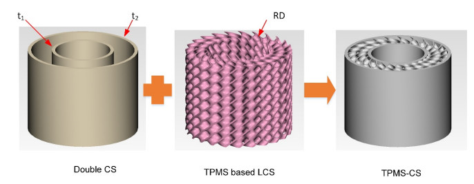
Cylinder shell (CS) structures are widely applied in marine industry applications with the characteristics of high loading ability and high energy absorption performance. In this study, the triply periodic minimal surfaces (TPMS) lattices were filled into double cylinder shell structures to construct the cylinder shell (TPMS-CS) structures. The mechanical and energy absorption performances of these structures were investigated by simulation analysis. First, the finite element (FE) model of TPMS-CS structures was verified by experiments. Then, the crashworthiness characteristics of three different kinds of TPMS-CS, namely, primitive, diamond, and gyroid, under axial loading were studied using FE simulation. The results indicate that the diamond-based TPMS-CS structures exhibit a higher energy absorption efficiency compared to their counterparts. Next, parametric studies were carried out to investigate the influence of the design parameters (the relative density of the TPMS, and the inner and outer shell thickness) on the crashworthiness of TPMS-CS structures. Finally, to obtain the optimum design for the TPMS-CS, an optimization framework was proposed by combining the three surrogate models (KGR, PRS, RBF) and multi-objective particle swarm optimization. The optimum design of the D-TPMS-CS structures was obtained based on the proposed optimization framework. The TPMS-CS structures proposed in this study can also be applied in other engineering applications as energy absorbers.
Citation: Laiyu Liang, Huaiming Zhu, Dong Wei, Yaozhong Wu, Weijia Li. Energy absorption and multi-objective optimization of TPMS filled cylinder shell structures[J]. Electronic Research Archive, 2023, 31(5): 2834-2854. doi: 10.3934/era.2023143
Cylinder shell (CS) structures are widely applied in marine industry applications with the characteristics of high loading ability and high energy absorption performance. In this study, the triply periodic minimal surfaces (TPMS) lattices were filled into double cylinder shell structures to construct the cylinder shell (TPMS-CS) structures. The mechanical and energy absorption performances of these structures were investigated by simulation analysis. First, the finite element (FE) model of TPMS-CS structures was verified by experiments. Then, the crashworthiness characteristics of three different kinds of TPMS-CS, namely, primitive, diamond, and gyroid, under axial loading were studied using FE simulation. The results indicate that the diamond-based TPMS-CS structures exhibit a higher energy absorption efficiency compared to their counterparts. Next, parametric studies were carried out to investigate the influence of the design parameters (the relative density of the TPMS, and the inner and outer shell thickness) on the crashworthiness of TPMS-CS structures. Finally, to obtain the optimum design for the TPMS-CS, an optimization framework was proposed by combining the three surrogate models (KGR, PRS, RBF) and multi-objective particle swarm optimization. The optimum design of the D-TPMS-CS structures was obtained based on the proposed optimization framework. The TPMS-CS structures proposed in this study can also be applied in other engineering applications as energy absorbers.

| [1] |
T. N. Doan, N. T. Thanh, P. Van Chuong, N. C. Tho, N. T. Ta, H. N. Nguyen, Analysis of stress concentration phenomenon of cylinder laminated shells using higher-order shear deformation Quasi-3D theory, Compos. Struct., 232 (2020), 111526. https://doi.org/10.1016/j.compstruct.2019.111526 doi: 10.1016/j.compstruct.2019.111526

|
| [2] |
P. Jiao, Z. Chen, H. Ma, P. Ge, Y. Gu, H. Miao, Buckling behaviors of thin-walled cylindrical shells under localized axial compression loads, Part 1: Experimental study, Thin-Walled Struct., 166 (2021), 108118. https://doi.org/10.1016/J.Tws.2021.108118 doi: 10.1016/J.Tws.2021.108118
|
| [3] |
H. Wagner, C. Hühne, M. Janssen, Buckling of cylindrical shells under axial compression with loading imperfections: An experimental and numerical campaign on low knockdown factors, Thin-Walled Struct., 151 (2020), 106764. https://doi.org/10.1016/J.Tws.2020.106764 doi: 10.1016/J.Tws.2020.106764
|
| [4] |
S. M. Hosseini, M. Shariati, Experimental analysis of energy absorption capability of thin-walled composite cylindrical shells by quasi-static axial crushing test, Thin-Walled Struct., 125 (2018), 259–268. https://doi.org/10.1016/j.tws.2018.01.026 doi: 10.1016/j.tws.2018.01.026
|
| [5] |
D. Karagiozova, N. Jones, Dynamic effects on buckling and energy absorption of cylindrical shells under axial impact, Thin-Walled Struct., 39 (2001), 583–610. https://doi.org/10.1016/S0263-8231(01)00015-5 doi: 10.1016/S0263-8231(01)00015-5
|
| [6] |
P. B. Su, B. Han, M. Yang, Z. H. Wei, Z. Y. Zhao, Q. C. Zhang, et al., Axial compressive collapse of ultralight corrugated sandwich cylindrical shells, Mater. Des., 160 (2018), 325–337. https://doi.org/10.1016/j.matdes.2018.09.034 doi: 10.1016/j.matdes.2018.09.034
|
| [7] |
H. Zhu, P. Wang, D. Wei, J. Si, Y. Wu, Energy absorption of diamond lattice cylindrical shells under axial compression loading, Thin-Walled Struct., 181 (2022), 110131. https://doi.org/10.1016/j.tws.2022.110131 doi: 10.1016/j.tws.2022.110131
|
| [8] |
Y. Wang, X. Ren, Z. Chen, Y. Jiang, X. Cao, S. Fang, et al., Numerical and experimental studies on compressive behavior of Gyroid lattice cylindrical shells, Mater. Des., 186 (2020), 108340. https://doi.org/10.1016/j.matdes.2019.108340 doi: 10.1016/j.matdes.2019.108340
|
| [9] |
H. Huang, Q. Han, Nonlinear elastic buckling and postbuckling of axially compressed functionally graded cylindrical shells, Int. J. Mech. Sci., 51 (2009), 500–507. https://doi.org/10.1016/j.ijmecsci.2009.05.002 doi: 10.1016/j.ijmecsci.2009.05.002
|
| [10] |
Y. Wu, L. Sun, P. Yang, J. Fang, W. Li, Energy absorption of additively manufactured functionally bi-graded thickness honeycombs subjected to axial loads, Thin-Walled Struct., 164 (2021), 107810. https://doi.org/10.1016/j.tws.2021.107810 doi: 10.1016/j.tws.2021.107810
|
| [11] |
J. Fang, G. Sun, N. Qiu, T. Pang, S. Li, Q. Li, On hierarchical honeycombs under out-of-plane crushing, Int. J. Solids Struct., 135 (2018), 1–13. https://doi.org/10.1016/j.ijsolstr.2017.08.013 doi: 10.1016/j.ijsolstr.2017.08.013
|
| [12] |
X. Niu, F. Xu, Z. Zou, T. Fang, S. Zhang, Q. Xie, In-plane dynamic crashing behavior and energy absorption of novel bionic honeycomb structures, Compos. Struct., 299 (2022), 116064. https://doi.org/10.1016/j.compstruct.2022.116064 doi: 10.1016/j.compstruct.2022.116064
|
| [13] |
X. Niu, F. Xu, Z. Zou, Bionic inspired honeycomb structures and multi-objective optimization for variable graded layers, J. Sandwich Struct. Mater., 25 (2023), 215–231. https://doi.org/10.1177/10996362221127969 doi: 10.1177/10996362221127969
|
| [14] |
M. F. Ashby, The properties of foams and lattices, Phil. Trans. R. Soc. A, 364 (2006), 15–30. https://doi.org/10.1098/rsta.2005.1678 doi: 10.1098/rsta.2005.1678
|
| [15] |
H. S. Abdulhadi, A. Mian, Effect of strut length and orientation on elastic mechanical response of modified body-centered cubic lattice structures, Proc. Inst. Mech. Eng., Part L: J. Mater.: Des. Appl., 233 (2019), 2219–2233. https://doi.org/10.1177/1464420719841084 doi: 10.1177/1464420719841084
|
| [16] |
Y. Wang, B. Ramirez, K. Carpenter, C. Naify, D. C. Hofmann, C. Daraio, Architected lattices with adaptive energy absorption, Extreme Mech. Lett., 33 (2019), 100557. https://doi.org/10.1016/J.Eml.2019.100557 doi: 10.1016/J.Eml.2019.100557
|
| [17] |
Y. Zhang, Z. Xue, L. Chen, D. Fang, Deformation and failure mechanisms of lattice cylindrical shells under axial loading, Int. J. Mech. Sci., 51 (2009), 213–221. https://doi.org/10.1016/j.ijmecsci.2009.01.006 doi: 10.1016/j.ijmecsci.2009.01.006
|
| [18] |
L. Chen, J. Zhang, B. Du, H. Zhou, H. Liu, Y. Guo, et al., Dynamic crushing behavior and energy absorption of graded lattice cylindrical structure under axial impact load, Thin-Walled Struct., 127 (2018), 333–343. https://doi.org/10.1016/j.tws.2017.10.048 doi: 10.1016/j.tws.2017.10.048
|
| [19] |
B. Du, L. Chen, W. Wu, H. Liu, Y. Zhao, S. Peng, et al., A novel hierarchical thermoplastic composite honeycomb cylindrical structure: Fabrication and axial compressive properties, Compos. Sci. Technol., 164 (2018), 136–145. https://doi.org/10.1016/j.compscitech.2018.05.021 doi: 10.1016/j.compscitech.2018.05.021
|
| [20] |
Y. Wu, J. Fang, C. Wu, C. Li, G. Sun, Q. Li, Additively manufactured materials and structures: A state-of-the-art review on their mechanical characteristics and energy absorption, Int. J. Mech. Sci., 246 (2023), 108102. https://doi.org/10.1016/j.ijmecsci.2023.108102 doi: 10.1016/j.ijmecsci.2023.108102
|
| [21] |
N. Qiu, J. Zhang, F. Yuan, Z. Jin, Y. Zhang, J. Fang, Mechanical performance of triply periodic minimal surface structures with a novel hybrid gradient fabricated by selective laser melting, Eng. Struct., 263 (2022), 114377. https://doi.org/10.1016/j.engstruct.2022.114377 doi: 10.1016/j.engstruct.2022.114377
|
| [22] |
L. Zhang, S. Feih, S. Daynes, S. Chang, M. Y. Wang, J. Wei, et al., Energy absorption characteristics of metallic triply periodic minimal surface sheet structures under compressive loading, Addit. Manuf., 23 (2018), 505–515. https://doi.org/10.1016/j.addma.2018.08.007 doi: 10.1016/j.addma.2018.08.007
|
| [23] |
N. Qiu, J. Zhang, C. Li, Y. Shen, J. Fang, Mechanical properties of three-dimensional functionally graded TPMS structures, Int. J. Mech. Sci., 246 (2023), 108118. https://doi.org/10.1016/j.ijmecsci.2023.108118 doi: 10.1016/j.ijmecsci.2023.108118
|
| [24] |
H. Yin, Z. Liu, J. Dai, G. Wen, C. Zhang, Crushing behavior and optimization of sheet-based 3D periodic cellular structures, Composites, Part B, 182 (2020), 107565. https://doi.org/10.1016/j.compositesb.2019.107565 doi: 10.1016/j.compositesb.2019.107565
|
| [25] |
O. Al-Ketan, R. K. Abu Al-Rub, Multifunctional mechanical metamaterials based on triply periodic minimal surface lattices, Adv. Eng. Mater., 21 (2019), 1900524. https://doi.org/10.1002/Adem.201900524 doi: 10.1002/Adem.201900524
|
| [26] |
H. Sun, C. Ge, Q. Gao, N. Qiu, L. Wang, Crashworthiness of sandwich cylinder filled with double-arrowed auxetic structures under axial impact loading, Int. J. Crashworthiness, 27 (2022), 1383–1392. https://doi.org/10.1080/13588265.2021.1947071 doi: 10.1080/13588265.2021.1947071
|
| [27] |
Y. Wu, J. Fang, Y. He, W. Li, Crashworthiness of hierarchical circular-joint quadrangular honeycombs, Thin-Walled Struct., 133 (2018), 180–191. https://doi.org/10.1016/j.tws.2018.09.044 doi: 10.1016/j.tws.2018.09.044
|
| [28] |
Y. Wu, J. Fang, Z. Cheng, Y. He, W. Li, Crashworthiness of tailored-property multi-cell tubular structures under axial crushing and lateral bending, Thin-Walled Struct., 149 (2020), 106640. https://doi.org/10.1016/j.tws.2020.106640 doi: 10.1016/j.tws.2020.106640
|
| [29] |
Y. Zhang, M. Lu, C. H. Wang, G. Sun, G. Li, Out-of-plane crashworthiness of bio-inspired self-similar regular hierarchical honeycombs, Compos. Struct., 144 (2016), 1–13. https://doi.org/10.1016/j.compstruct.2016.02.014 doi: 10.1016/j.compstruct.2016.02.014
|
| [30] |
G. Sun, S. Li, Q. Liu, G. Li, Q. Li, Experimental study on crashworthiness of empty/aluminum foam/honeycomb-filled CFRP tubes, Compos. Struct., 152 (2016), 969–993. https://doi.org/10.1016/j.compstruct.2016.06.019 doi: 10.1016/j.compstruct.2016.06.019
|
| [31] |
J. Fang, G. Sun, N. Qiu, N. H. Kim, Q. Li, On design optimization for structural crashworthiness and its state of the art, Struct. Multidiscip. Optim., 55 (2017), 1091–1119. https://doi.org/10.1007/s00158-016-1579-y doi: 10.1007/s00158-016-1579-y
|
| [32] |
J. Fang, Y. Gao, G. Sun, G. Zheng, Q. Li, Dynamic crashing behavior of new extrudable multi-cell tubes with a functionally graded thickness, Int. J. Mech. Sci., 103 (2015), 63–73. https://doi.org/10.1016/j.ijmecsci.2015.08.029 doi: 10.1016/j.ijmecsci.2015.08.029
|
| [33] |
G. Sun, T. Pang, J. Fang, G. Li, Q. Li, Parameterization of criss-cross configurations for multiobjective crashworthiness optimization, Int. J. Mech. Sci., 124 (2017), 145–157. https://doi.org/10.1016/j.ijmecsci.2017.02.027 doi: 10.1016/j.ijmecsci.2017.02.027
|
| [34] |
J. S. Park, Optimal Latin-hypercube designs for computer experiments, J. Stat. Plann. Inference, 39 (1994), 95–111. https://doi.org/10.1016/0378-3758(94)90115-5 doi: 10.1016/0378-3758(94)90115-5
|
| [35] |
N. Qiu, Y. Gao, J. Fang, Z. Feng, G. Sun, Q. Li, Crashworthiness analysis and design of multi-cell hexagonal columns under multiple loading cases, Finite Elem. Anal. Des., 104 (2015), 89–101. https://doi.org/10.1016/j.finel.2015.06.004 doi: 10.1016/j.finel.2015.06.004
|
| [36] |
Y. Wu, W. Li, J. Fang, Q. Lan, Multi-objective robust design optimization of fatigue life for a welded box girder, Eng. Optim., 50 (2018), 1252–1269. https://doi.org/10.1080/0305215X.2017.1395023 doi: 10.1080/0305215X.2017.1395023
|
| [37] |
X. Song, G. Sun, G. Li, W. Gao, Q. Li, Crashworthiness optimization of foam-filled tapered thin-walled structure using multiple surrogate models, Struct. Multidiscip. Optim., 47 (2013), 221–231. https://doi.org/10.1007/s00158-012-0820-6 doi: 10.1007/s00158-012-0820-6
|
| [38] |
H. M. Gutmann, A radial basis function method for global optimization, J. Global Optim, 19 (2001), 201–227. https://doi.org/10.1023/A:1011255519438 doi: 10.1023/A:1011255519438
|
| [39] |
A. I. J. Forrester, A. J. Keane, Recent advances in surrogate-based optimization, Prog. Aerosp. Sci., 45 (2009), 50–79. https://doi.org/10.1016/j.paerosci.2008.11.001 doi: 10.1016/j.paerosci.2008.11.001
|
| [40] |
J. Fu, Q. Liu, K. Liufu, Y. Deng, J. Fang, Q. Li, Design of bionic-bamboo thin-walled structures for energy absorption, Thin-Walled Struct., 135 (2019), 400–413. https://doi.org/10.1016/j.tws.2018.10.003 doi: 10.1016/j.tws.2018.10.003
|
| [41] |
N. Qiu, Z. Jin, J. Liu, L. Fu, Z. Chen, N. H. Kim, Hybrid multi-objective robust design optimization of a truck cab considering fatigue life, Thin-Walled Struct., 162 (2021), 107545. https://doi.org/10.1016/j.tws.2021.107545 doi: 10.1016/j.tws.2021.107545
|
| [42] |
C. A. C. Coello, G. T. Pulido, M. S. Lechuga, Handling multiple objectives with particle swarm optimization, IEEE Trans. Evol. Comput., 8 (2004), 256–279. https://doi.org/10.1109/TEVC.2004.826067 doi: 10.1109/TEVC.2004.826067
|
| [43] |
J. Fang, Y. Gao, G. Sun, N. Qiu, Q. Li, On design of multi-cell tubes under axial and oblique impact loads, Thin-Walled Struct., 95 (2015), 115–126. https://doi.org/10.1016/j.tws.2015.07.002 doi: 10.1016/j.tws.2015.07.002
|


Figures(12) / Tables(9)
Laiyu Liang, Huaiming Zhu, Dong Wei, Yaozhong Wu, Weijia Li. Energy absorption and multi-objective optimization of TPMS filled cylinder shell structures[J]. Electronic Research Archive, 2023, 31(5): 2834-2854. doi: 10.3934/era.2023143


 DownLoad: