Tapping stream tracking model using computer vision and deep learning to minimize slag carry-over in basic oxygen furnace

Dae-Geun Hong; Woong-Hee Han; Chang-Hee Yim; Dae-Geun Hong; Woong-Hee Han; Chang-Hee Yim

doi:10.3934/era.2022204

Electronic Research Archive

2022, Volume 30, Issue 11: 4015-4037. doi: 10.3934/era.2022204

Previous Article Next Article

Research article Special Issues

Tapping stream tracking model using computer vision and deep learning to minimize slag carry-over in basic oxygen furnace

1.
Graduate Institute of Ferrous and Energy Materials Technology, Pohang University of Science and Technology, 77 Cheongam-Ro, Nam-Gu, Pohang, Gyeongbuk 37673, Republic of Korea
2.
Steel Making Research Group, POSCO Research Institute, 8 Pokposarang-gil, Gwangyang-si, Jeollanam-do 57807, Republic of Korea

Received: 02 June 2022 Revised: 04 August 2022 Accepted: 23 August 2022 Published: 13 September 2022

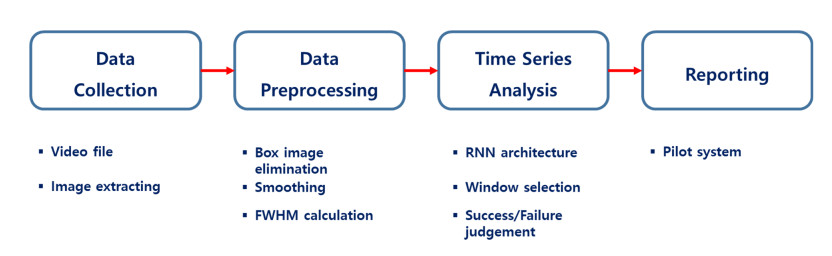
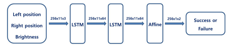
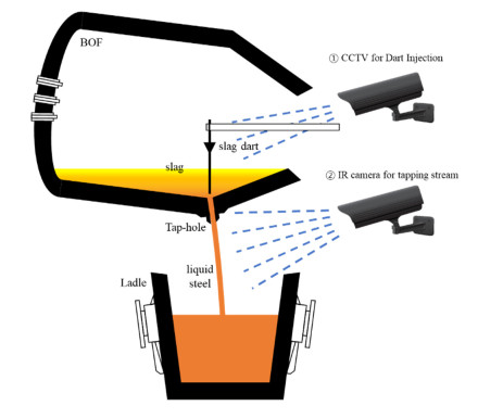
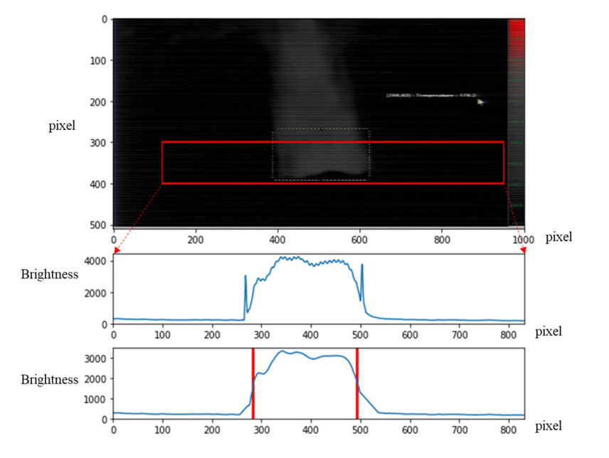
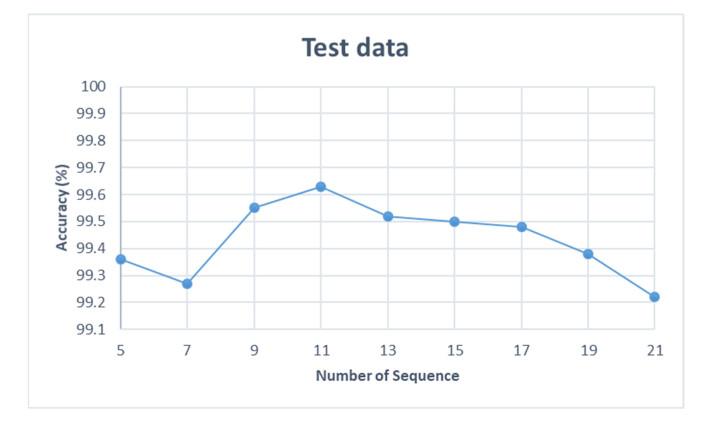
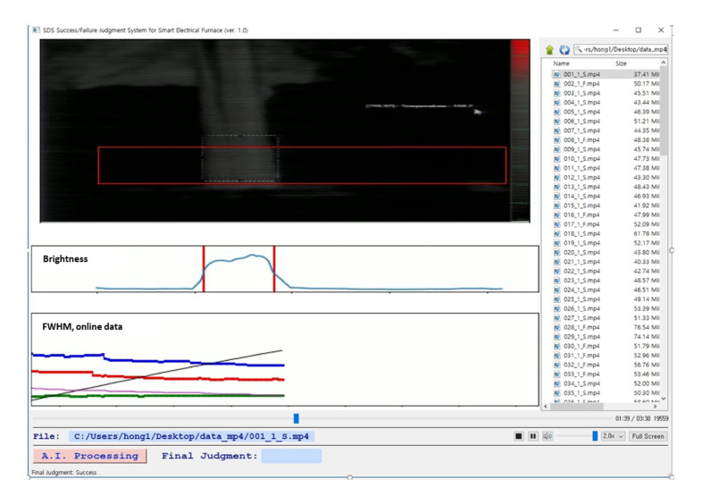
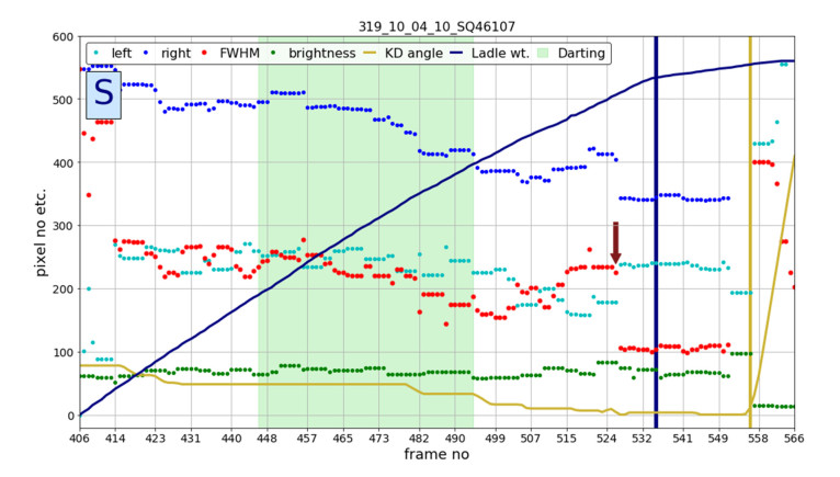
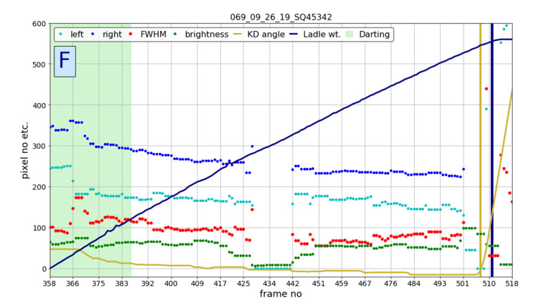
This paper describes a system that can automatically determine the result of the slag dart input to the converter during tapping of basic oxygen furnace (BOF), by directly observing and tracking the behavior of the pouring molten steel at the tapping hole after the dart is injected. First, we propose an algorithm that detects and tracks objects, then automatically calculates the width of the tapping stream from slag-detection system (SDS) images collected in real time. Second, we develop a time-series model that can determine whether the slag dart was properly seated on the tap hole; this model uses the sequential width and brightness data of the tapping stream. To test the model accuracy, an experiment was performed using SDS data collected in a real BOF. When the number of sequential images was 11 and oversampling was 2:1, the classification accuracy in the test data set was 99.61%. Cases of success and failure of dart injection were quantified in connection with operation data such as ladle weight and tilt angle. A pilot system was constructed; it increases the reliability of prevention of slag carry-over during tapping, and can reduce the operator's workload by as much as 30%. This system can reduce the secondary refining cost by reducing the dart-misclassification rate, and thereby increase the productivity of the steel mill. Finally, the system can contribute to real-time process control and management by automatically linking the task of determining the input of darts to the work of minimizing slag carry-over in a BOF.

Keywords:

Citation: Dae-Geun Hong, Woong-Hee Han, Chang-Hee Yim. Tapping stream tracking model using computer vision and deep learning to minimize slag carry-over in basic oxygen furnace[J]. Electronic Research Archive, 2022, 30(11): 4015-4037. doi: 10.3934/era.2022204

Related Papers:

[1]	Ruizhi Yang, Dan Jin, Wenlong Wang . A diffusive predator-prey model with generalist predator and time delay. AIMS Mathematics, 2022, 7(3): 4574-4591. doi: 10.3934/math.2022255
[2]	Yingyan Zhao, Changjin Xu, Yiya Xu, Jinting Lin, Yicheng Pang, Zixin Liu, Jianwei Shen . Mathematical exploration on control of bifurcation for a 3D predator-prey model with delay. AIMS Mathematics, 2024, 9(11): 29883-29915. doi: 10.3934/math.20241445
[3]	Sahabuddin Sarwardi, Hasanur Mollah, Aeshah A. Raezah, Fahad Al Basir . Direction and stability of Hopf bifurcation in an eco-epidemic model with disease in prey and predator gestation delay using Crowley-Martin functional response. AIMS Mathematics, 2024, 9(10): 27930-27954. doi: 10.3934/math.20241356
[4]	Xin-You Meng, Fan-Li Meng . Bifurcation analysis of a special delayed predator-prey model with herd behavior and prey harvesting. AIMS Mathematics, 2021, 6(6): 5695-5719. doi: 10.3934/math.2021336
[5]	Heping Jiang . Complex dynamics induced by harvesting rate and delay in a diffusive Leslie-Gower predator-prey model. AIMS Mathematics, 2023, 8(9): 20718-20730. doi: 10.3934/math.20231056
[6]	Qinghui Liu, Xin Zhang . Chaos detection in predator-prey dynamics with delayed interactions and Ivlev-type functional response. AIMS Mathematics, 2024, 9(9): 24555-24575. doi: 10.3934/math.20241196
[7]	Hairong Li, Yanling Tian, Ting Huang, Pinghua Yang . Hopf bifurcation and hybrid control of a delayed diffusive semi-ratio-dependent predator-prey model. AIMS Mathematics, 2024, 9(10): 29608-29632. doi: 10.3934/math.20241434
[8]	Fatao Wang, Ruizhi Yang, Yining Xie, Jing Zhao . Hopf bifurcation in a delayed reaction diffusion predator-prey model with weak Allee effect on prey and fear effect on predator. AIMS Mathematics, 2023, 8(8): 17719-17743. doi: 10.3934/math.2023905
[9]	Eric M. Takyi, Charles Ohanian, Margaret Cathcart, Nihal Kumar . Sex-biased predation and predator intraspecific competition effects in a prey mating system. AIMS Mathematics, 2024, 9(1): 2435-2453. doi: 10.3934/math.2024120
[10]	Liye Wang, Wenlong Wang, Ruizhi Yang . Stability switch and Hopf bifurcations for a diffusive plankton system with nonlocal competition and toxic effect. AIMS Mathematics, 2023, 8(4): 9716-9739. doi: 10.3934/math.2023490

Abstract

1. Introduction

In survey sampling, it is well known fact that suitable use of the auxiliary information may improves the precision of an estimator for the unknown population parameters. The auxiliary information can be used either at the design stage or at estimation stage to increase the accuracy of the population parameter estimators. Several authors presented modified different type of estimators for estimating the finite population mean including ^{[4,9,21,22,23,24,25,26,27]}.

The problem of estimation of finite population mean or total in two-stage sampling scheme using the auxiliary information has been well established. The two stage sampling scheme is an improvement over the cluster sampling, when it is not possible or easy to calculate all the units from the selected clusters. One of the main characteristic could be the budget, and it becomes too difficult to collect information from all the units within the selected clusters. To overcome this, one way is to select clusters, called first stage unit (fsus) and from the given population of interest, select a subsample from the selected clusters called the second stage units (ssu). This also benefits to increase the size of the first stage samples which consist of clusters, and assume to be heterogeneous groups. If there is no variation within clusters then might not be possible to collect information from all the units within selected clusters. In many situations, it is not possible to obtain the complete list of ultimate sampling units in large scale sample surveys, while a list of primary units of clusters may be available. In such situations, we select a random sample of first stage units or primary units using certain probability sampling schemes i.e simple random sampling (with or without replacement), systematic sampling and probability proportional to size (PPS), and then we can perform sub-sampling in selected clusters (first stage units). This approach is called two-stage sampling scheme.

Two-stage has a great varaity of applications, which go far beyond the immediate scop of sample survey. Whenever any process involves in chemical, physical, or biological tests that can be performed on a small amount of materail, it is likely to be drawn as a subsample from a larger amount that is itself a sample.

In large scale survey sampling, it is usual to adopt multistage sampling to estimate the population mean or total of the study variable $y$ . ^[13] proposed a general class of estimators of a finite population mean using multi-auxiliary information under two stage sampling scheme. ^[1] proposed an alternative class of estimators in two stage sampling with two auxiliary variables. ^[10] proposed estimators for finite population mean under two-stage sampling using multivariate auxiliary information. ^[12] suggested a detailed note on ratio estimates in multi-stage sampling. ^[6] given some stratagies in two stage sampling using auxiliary information. ^[3] suggested a class of predictive estimaotrs in two stage sampling using auxiliary information. ^[8] gave a generalized method of estimation for two stage sampling using two auxiliary variables. ^[5] suggested chain ratio estimators in two stage sampling. For certain related work, we refer some latest articles, i.e., ^{[14,15,16,17,18,19,20]}.

In this article, we propose an improved generalized class of estimators using two auxiliary variables under two-stage sampling scheme. The biases and mean sqaure errors of the proposed generalized class of estimators are derived up to first order of approximation. Based on the numerical results, the proposed class of estimators are more efficient than their existing counterparts.

2. Symbols and notation

Consider a finite population $U$ = $\{{U}_{1}, {U}_{2}, ..., {U}_{N}\}$ is divided into $N$ first-stage units (fsus) clusters in the population. Let N be the total number of first stage unit in population, n be the number of first stage units selected in the sample, ${M}_{i}$ be the number of second stage units (ssus) belongs to the ${i}^{th}$ first stage units (fsus), (i = 1, 2, …, N), and mi be the number of fsus selected from the ${i}^{th}$ fsu in the sample of n fsus, (i = 1, 2, …, n).

Let ${y}_{ij}$ , ${x}_{ij}$ and ${z}_{ij}$ be values of the study variable $y$ and the auxiliary variables $\left(x\mathrm{a}\mathrm{n}\mathrm{d}z\right)$ respectively, for the ${j}^{th}$ ssus ${U}_{i} = (j = \mathrm{1, 2}, ..., {M}_{i})$ , in the ${i}^{th}$ fsus. The population mean of the study variable $y$ and the auxiliary variables $(x, z)$ are given by:

$\overline {Y} = \frac{1}{N}\sum _{i = 1}^{N}\;{u}_{i}{\overline {Y}}_{i}, \;\;\;\;\overline {X} = \frac{1}{N}\sum _{i = 1}^{N}\;{u}_{i}{\overline {X}}_{i}, \;\;\;\;\overline {Z} = \frac{1}{N}\sum _{i = 1}^{N}\;{u}_{i}{\overline {Z}}_{i} ,$

where

${\overline {Y}}_{i} = \frac{1}{{M}_{i}}\sum\limits_{j = 1}^{{M}_{i}}\;{y}_{ij}, {\overline {X}}_{i} = \frac{1}{{M}_{i}}\sum\limits_{j = 1}^{{M}_{i}}\;{x}_{ij}, {\overline {Z}}_{i} = \frac{1}{{M}_{i}}\sum\limits_{j = 1}^{{M}_{i}}\;{z}_{ij}, \;\;(i = \mathrm{1, 2}, ..., N).$

${u}_{i} = \frac{{M}_{i}}{\overline {M}} , \;{\rm{and}}\; \overline {M} = \frac{M}{N} , \; M = \sum _{i = 1}^{N}\;{M}_{i} ,$

$R = \frac{\overline {Y}}{\overline {X}} , \; {\rm{and}} \; {R}_{i} = \frac{{\overline {Y}}_{i}}{{\overline {X}}_{i}} ,$

${S}_{by}^{2} = \frac{1}{N-1}\sum _{i = 1}^{N}\;({u}_{i}{\overline {Y}}_{i}-\overline {Y}{)}^{2} ,$

${S}_{bx}^{2} = \frac{1}{N-1}\sum _{i = 1}^{N}\;({u}_{i}{\overline {X}}_{i}-\overline {X}{)}^{2} ,$

${S}_{bz}^{2} = \frac{1}{N-1}\sum _{i = 1}^{N}\;({u}_{i}{\overline {Z}}_{i}-\overline {Z}{)}^{2} ,$

${S}_{byx} = \frac{1}{N-1}\sum _{i = 1}^{N}\;\left({u}_{i}{\overline {Y}}_{i}-\overline {Y}\right)\left({u}_{i}{\overline {X}}_{i}-\overline {X}\right), \;\;\;\;\;\;\;\;{S}_{byz} = \frac{1}{N-1}\sum _{i = 1}^{N}\;({u}_{i}{\overline {Z}}_{i}-\overline {Z})({u}_{i}{\overline {Y}}_{i}-\overline {Y}) ,$

${S}_{bxz} = \frac{1}{N-1}\sum _{i = 1}^{N}\;({u}_{i}{\overline {Z}}_{i}-\overline {Z})({u}_{i}{\overline {X}}_{i}-\overline {X}), \;\;\;\;\;\;\;\;{S}_{iy}^{2} = \frac{1}{{M}_{i}-1}\sum _{j = 1}^{{M}_{i}}\;({y}_{ij}-{\overline {Y}}_{i}{)}^{2} ,$

${S}_{ix}^{2} = \frac{1}{{M}_{i}-1}\sum _{j = 1}^{{M}_{i}}\;({x}_{ij}-{\overline {X}}_{i}{)}^{2}, \;\;\;\;\;\;\;\;{S}_{iz}^{2} = \frac{1}{{M}_{i}-1}\sum _{j = 1}^{{M}_{i}}\;({z}_{ij}-{\overline {Z}}_{i}{)}^{2} ,$

${S}_{iyx} = \frac{1}{{M}_{i}-1}({y}_{ij}-{\overline {Y}}_{i})({x}_{ij}-{\overline {X}}_{i}), \;\;\;\;\;\;\;\;{S}_{iyz} = \frac{1}{{M}_{i}-1}({y}_{ij}-{\overline {Y}}_{i})({z}_{ij}-{\overline {Z}}_{i}) ,$

${S}_{ixz} = \frac{1}{{M}_{i}-1}\sum\limits_{j = 1}^{{M}_{i}}\;({x}_{ij}-{\overline {X}}_{i})({z}_{ij}-{\overline {Z}}_{i}), \;\;\;\;\;\;\;\;(i = \mathrm{1, 2}, ...N).$

Similarly for sample data:

$\overline {y} = \frac{1}{n}\sum _{i = 1}^{n}\;{u}_{i}{\overline {y}}_{i} = {\overline {y}}^{\mathrm{*}}\left(say\right), \;\overline {x} = \frac{1}{n}\sum _{i = 1}^{n}\;{u}_{i}{\overline {x}}_{i} = {\overline {x}}^{\mathrm{*}}\left(say\right), \;\overline {z} = \frac{1}{n}\sum _{i = 1}^{n}\;{u}_{i}{\overline {z}}_{i} = {\overline {z}}^{\mathrm{*}}\left(say\right),$

where

${\overline {y}}_{i} = \frac{1}{{m}_{i}}\sum\limits_{j = 1}^{{m}_{i}}\;{y}_{ij}, \;\;\;\;{\overline {x}}_{i} = \frac{1}{{m}_{i}}\sum\limits_{j = 1}^{{m}_{i}}\;{x}_{ij}, \;\;\;\;{\overline {z}}_{i} = \frac{1}{{m}_{i}}\sum\limits_{j = 1}^{{m}_{i}}\;{z}_{ij},$

${s}_{by}^{2} = \frac{1}{n-1}\sum _{i = 1}^{n}\;({u}_{i}{\overline {y}}_{i}-\overline {y}{)}^{2}, \;\;\;\;\;\;\;\;{s}_{bx}^{2} = \frac{1}{n-1}\sum _{i = 1}^{n}\;({u}_{i}{\overline {x}}_{i}-\overline {x}{)}^{2} ,$

${s}_{bz}^{2} = \frac{1}{n-1}\sum _{i = 1}^{n}\;({u}_{i}{\overline {z}}_{i}-\overline {z}{)}^{2}, \;\;\;\;\;\;\;\;{s}_{byx} = \frac{1}{n-1}\sum _{i = 1}^{n}\;({u}_{i}{\overline {y}}_{i}-\overline {y}\left)\right({u}_{i}{\overline {x}}_{i}-\overline {x}) ,$

${s}_{byz} = \frac{1}{n-1}\sum _{i = 1}^{n}\;({u}_{i}{\overline {y}}_{i}-\overline {y})({u}_{i}{\overline {z}}_{i}-\overline {z}), \;\;\;\;\;\;\;\;{s}_{bxz} = \frac{1}{n-1}\sum _{i = 1}^{n}\;({u}_{i}{\overline {x}}_{i}-\overline {x})({u}_{i}{\overline {z}}_{i}-\overline {z}) ,$

${s}_{iy}^{2} = \frac{1}{{m}_{i}-1}({y}_{ij}-{\overline {y}}_{i}{)}^{2}, \;\;\;\;\;\;\;\;{s}_{ix}^{2} = \frac{1}{{m}_{i}-1}({x}_{ij}-{\overline {x}}_{i}{)}^{2} ,$

${s}_{iz}^{2} = \frac{1}{{m}_{i}-1}({z}_{ij}-{\overline {z}}_{i}{)}^{2}, \;\;\;\;\;\;\;\;{s}_{iyx} = \frac{1}{{m}_{i}-1}\sum _{j = 1}^{{m}_{i}}\;({y}_{ij}-{\overline {y}}_{i}\left)\right({x}_{ij}-{\overline {x}}_{i}) ,$

${s}_{iyz} = \frac{1}{{m}_{i}-1}\sum _{j = 1}^{{m}_{i}}\;\left({y}_{ij}-{\overline {y}}_{i}\right)\left({z}_{ij}-{\overline {z}}_{i}\right), \;\;\;\;\;\;\;\;{s}_{ixz} = \frac{1}{{m}_{i}-1}\sum _{j = 1}^{{m}_{i}}\;({x}_{ij}-{\overline {x}}_{i})({z}_{ij}-{\overline {z}}_{i}) .$

In order to obtain the biases and mean sqaured errors, we consider the following relative error terms:

${e}_{0} = \frac{{\overline {y}}^{\mathrm{*}}-\overline {Y}}{\overline {Y}}, \;{e}_{1} = \frac{{\overline {x}}^{\mathrm{*}}-\overline {X}}{\overline {X}}, \;{e}_{2} = \frac{{\overline {z}}^{\mathrm{*}}-\overline {Z}}{\overline {Z}} ,$

$E\left({e}_{0}^{2}\right) = \lambda {C}_{by}^{2}+\frac{1}{nN}\sum _{i = 1}^{n}\;{u}_{i}^{2}{\theta }_{i}{C}_{iy}^{2} = {V}_{y} ,$

$E\left({e}_{1}^{2}\right) = \lambda {C}_{bx}^{2}+\frac{1}{nN}\sum _{i = 1}^{n}\;{u}_{i}^{2}{\theta }_{i}{C}_{ix}^{2} = {V}_{x} ,$

$E\left({e}_{2}^{2}\right) = \lambda {C}_{bz}^{2}+\frac{1}{nN}\sum _{i = 1}^{n}\;{u}_{i}^{2}{\theta }_{i}{C}_{iz}^{2} = {V}_{z} ,$

$E\left({e}_{0}{e}_{1}\right) = \lambda {C}_{byx}+\frac{1}{nN}\sum _{i = 1}^{n}\;{u}_{i}^{2}{\theta }_{i}{C}_{iyx} = {V}_{yx},$

$E\left({e}_{0}{e}_{2}\right) = \lambda {C}_{byz}+\frac{1}{nN}\sum _{i = 1}^{n}\;{u}_{i}^{2}{\theta }_{i}{C}_{iyz} = {V}_{yz},$

$E\left({e}_{1}{e}_{2}\right) = \lambda {C}_{bxz}+\frac{1}{nN}\sum _{i = 1}^{n}\;{u}_{i}^{2}{\theta }_{i}{C}_{ixz} = {V}_{xz} ,$

${C}_{by} = \frac{{S}_{by}}{\overline {Y}}, \;\;\;\;\;\;\;\;{C}_{bx} = \frac{{S}_{bx}}{\overline {X}}, \;\;\;\;\;\;\;\;{C}_{bz} = \frac{{S}_{bz}}{\overline {Z}} ,$

${C}_{byx} = \frac{{S}_{byx}}{\overline {Y}\overline {X}}, \;\;\;\;\;\;\;\;{C}_{byz} = \frac{{S}_{byz}}{\overline {Y}\overline {Z}}, \;\;\;\;\;\;\;\;{C}_{bxz} = \frac{{S}_{bxz}}{\overline {X}\overline {Z}} ,$

${C}_{iyx} = \frac{{S}_{iyx}}{\overline {Y}\overline {X}}, \;\;\;\;\;\;\;\;{C}_{iyz} = \frac{{S}_{byz}}{\overline {Y}\overline {Z}}, \;\;\;\;\;\;\;\;{C}_{ixz} = \frac{{S}_{ixz}}{\overline {X}\overline {Z}} ,$

${C}_{iy} = \frac{{S}_{iy}}{\overline {Y}}, \;\;\;\;\;\;\;\;{C}_{ix} = \frac{{S}_{ix}}{\overline {X}}, \;\;\;\;\;\;\;\;{C}_{iz} = \frac{{S}_{iz}}{\overline {Z}} ,$

where,

${\theta }_{i} = \left(\frac{1}{{m}_{i}}-\frac{1}{{M}_{i}}\right), \lambda = (\frac{1}{n}-\frac{1}{N}) .$

3. Existing estimators

In this section, we consider several estimators of the finite population mean under two-stage sampling that are available in the sampling literature, the properties of all estimators considered here are obtained up-to the first order of approximation.

(ⅰ) The usual mean estimator ${\overline {y}}^{\mathrm{*}} = {\overline {y}}_{0}^{\mathrm{*}}$ and its variance under two-stage sampling are given by:

${\overline {y}}_{0}^{\mathrm{*}} = \frac{1}{n}\sum _{i = 1}^{n}\;{u}_{i}{\overline {y}}_{i} ,$

(1)

and

$V\left({\overline {y}}_{0}^{\mathrm{*}}\right) = {\overline {Y}}^{2}{V}_{y} = MSE\left({\overline {y}}_{0}^{\mathrm{*}}\right) .$

(2)

(ⅱ) The usual ratio estimator under two-stage sampling, is given by:

${\overline {y}}_{R}^{\mathrm{*}} = {\overline {y}}^{\mathrm{*}}\left(\frac{\overline {X}}{{\overline {x}}^{\mathrm{*}}}\right) ,$

(3)

where $\overline {X}$ is the known population mean of $x$ .

The bias and $\mathrm{M}\mathrm{S}\mathrm{E}$ of ${\overline {y}}_{R}^{\mathrm{*}}$ to first order of approximation, are given by:

$Bias\left({\overline {y}}_{R}^{\mathrm{*}}\right) = \overline {Y}\left[{V}_{x}-{V}_{yx}\right] ,$

(4)

and

$MSE\left({\overline {y}}_{R}^{\mathrm{*}}\right) = {\overline {Y}}^{2}\left[{V}_{y}+{V}_{x}-2{V}_{yx}\right] .$

(5)

(ⅲ) ^[2] Exponential ratio type estimator under two-stage sampling, is given by:

${\overline {y}}_{E}^{\mathrm{*}} = {\overline {y}}^{\mathrm{*}}exp\left(\frac{\overline {X}-{\overline {x}}^{\mathrm{*}}}{\overline {X}+{\overline {x}}^{\mathrm{*}}}\right) .$

(6)

The bias and $MSE$ of ${\overline {y}}_{E}^{\mathrm{*}}$ to first order of approximation, are given by:

$Bias\left({\overline {y}}_{E}^{\mathrm{*}}\right) = \overline {Y}\left[\frac{3}{8}{V}_{x}-\frac{1}{2}{V}_{yx}\right] ,$

(7)

and

$MSE\left({\overline {y}}_{E}^{\mathrm{*}}\right) = {\overline {Y}}^{2}\left[{V}_{y}+\frac{1}{4}{V}_{x}-{V}_{yx}\right] .$

(8)

(ⅳ) The traditional difference estimator under two-stage sampling is given by:

${\overline {y}}_{D}^{\mathrm{*}} = {\overline {y}}^{\mathrm{*}}+d\left(\overline {X}-{\overline {x}}^{\mathrm{*}}\right) ,$

(9)

where $d$ is the constant.

The minimum variance of ${\overline {y}}_{D}^{\mathrm{*}}$ , is given by:

$V\left({\overline {y}}_{Dmin}^{\mathrm{*}}\right) = {\overline {Y}}^{2}{V}_{y}\left(1-{\rho }^{\mathrm{*}2}\right) = MSE\left({\overline {y}}_{D}^{\mathrm{*}}\right) ,$

(10)

where ${\rho }^{\mathrm{*}} = \frac{{V}_{yx}}{\sqrt{{V}_{y}}\sqrt{{V}_{x}}}$ .

The optimum value of $d$ is ${d}_{opt} = \frac{\overline {Y}{V}_{yx}}{\overline {X}{V}_{x}}$ .

(ⅴ) ^[7] Difference type estimator under two-stage sampling, is given by:

${\overline {y}}_{Rao}^{\mathrm{*}} = {d}_{0}{\overline {y}}^{\mathrm{*}}+{d}_{1}\left(\overline {X}-{\overline {x}}^{\mathrm{*}}\right) ,$

(11)

where ${d}_{0}$ and ${d}_{1}$ are constants.

The bias and minimum $\mathrm{M}\mathrm{S}\mathrm{E}$ of ${\overline {y}}_{Rao}^{\mathrm{*}}$ to first order of approximation, is given by:

$Bias\left({\overline {y}}_{Rao}^{\mathrm{*}}\right) = ({d}_{0}-1)\overline {Y} ,$

(12)

and

$MSE({\overline {y}}_{Rao}^{\mathrm{*}}{)}_{min}\cong \frac{{\overline {Y}}^{2}({V}_{x}{V}_{y}-{V}_{yx}^{2})}{{V}_{x}{V}_{y}-{V}_{yx}^{2}+{V}_{x}} = \frac{{\overline {Y}}^{2}{V}_{y}(1-{\rho }^{\mathrm{*}2})}{1+{V}_{y}(1-{\rho }^{\mathrm{*}2})} .$

(13)

The optimum values of ${d}_{0}$ and ${d}_{1}$ are:

${d}_{0opt} = \frac{{V}_{x}}{{V}_{x}{V}_{y}-{V}_{yx}^{2}+{V}_{x}}$ and ${d}_{1opt} = \frac{\overline {Y}{V}_{yx}}{\overline {X}({V}_{x}{V}_{y}-{V}_{yx}^{2}+{V}_{x})}$ .

(ⅵ) The difference-in-ratio type estimator under two-stage sampling, is given by:

${\overline {y}}_{DR}^{\mathrm{*}} = \left[{d}_{2}{\overline {y}}^{\mathrm{*}}+{d}_{3}(\overline {X}-{\overline {x}}^{\mathrm{*}})\right]\left(\frac{\overline {X}}{{\overline {x}}^{\mathrm{*}}}\right) ,$

(14)

where ${d}_{2}$ and ${d}_{3}$ are constants.

The bias and minimum $\mathrm{M}\mathrm{S}\mathrm{E}$ of ${\overline {y}}_{DR}^{\mathrm{*}}$ to first order of approximation, are given by:

$Bias\left({\overline {y}}_{DR}^{\mathrm{*}}\right)\cong \overline {Y}({d}_{2}-1)-{d}_{2}\overline {Y}{V}_{yx}+{d}_{3}\overline {X}{V}_{x}+{d}_{2}{V}_{x}\overline {Y} ,$

(15)

and

$MSE({\overline {y}}_{DR}^{\mathrm{*}}{)}_{min}\cong \frac{{\overline {Y}}^{2}({V}_{x}^{2}{V}_{y}-{V}_{x}{V}_{yx}^{2}-{V}_{x}{V}_{y}+{V}_{yx}^{2})}{({V}_{x}^{2}-{V}_{x}{V}_{y}+{V}_{yx}^{2}-{V}_{x})} .$

(16)

The optimum values of ${d}_{2}$ and ${d}_{3}$ are:

${d}_{2opt} = \frac{{V}_{x}({V}_{x}-1)}{{V}_{x}^{2}-{V}_{x}{V}_{y}+{V}_{yx}^{2}-{V}_{x}} ,$

${d}_{3opt} = \frac{-{\overline {Y}}^{2}({V}_{x}^{2}+{V}_{x}{V}_{y}-{V}_{x}{V}_{yx}-{V}_{yx}^{2}-{V}_{x}+{V}_{yx})}{\overline {X}({V}_{x}^{2}-{V}_{x}{V}_{y}+{V}_{yx}^{2}-{V}_{x})} .$

(ⅶ) The difference-in-exponential ratio type estimator under two-stage sampling, is given by:

${\overline {y}}_{DE}^{\mathrm{*}} = \left[{d}_{4}{\overline {y}}^{\mathrm{*}}+{d}_{5}(\overline {X}-{\overline {x}}^{\mathrm{*}})\right]\mathrm{e}\mathrm{x}\mathrm{p}\left(\frac{\overline {X}-{\overline {x}}^{\mathrm{*}}}{\overline {X}-{\overline {x}}^{\mathrm{*}}}\right) ,$

(17)

where ${d}_{4}$ and ${d}_{5}$ are constants.

The bias and minimum $\mathrm{M}\mathrm{S}\mathrm{E}$ of ${\overline {y}}_{DE}^{\mathrm{*}}$ to first order of approximation, are given by:

$Bias\left({\overline {y}}_{DE}^{\mathrm{*}}\right) = ({d}_{4}-1)\overline {Y}-\frac{1}{2}{d}_{4}\overline {Y}{V}_{yx}+\frac{3}{8}{d}_{4}\overline {Y}{V}_{x}+\frac{1}{2}{d}_{5}{V}_{x} ,$

(18)

and

$MSE({\overline {y}}_{DE}^{\mathrm{*}}{)}_{min}\cong \frac{-{\overline {Y}}^{2}\left({V}_{x}^{3}+16{V}_{x}^{2}{V}_{y}-16{V}_{x}{V}_{yx}^{2}-64{V}_{x}{V}_{y}+64{V}_{yx}^{2}\right)}{64{V}_{x}{V}_{y}-64{V}_{yx}^{2}+64{V}_{x}} .$

(19)

The optimum values of ${d}_{4}$ and ${d}_{5}$ are:

${d}_{4opt} = -\frac{1}{8}\frac{{V}_{x}({V}_{x}-8)}{({V}_{x}{V}_{y}-{V}_{yx}^{2}+{V}_{x})} ,$

${d}_{5opt} = \frac{\overline {Y}\left({V}_{x}^{2}+4{V}_{x}{V}_{y}-{V}_{x}{V}_{yx}-4{V}_{yx}^{2}-4{V}_{x}+8{V}_{yx}\right)}{\frac{1}{8}\overline {X}({V}_{x}{V}_{y}-{V}_{yx}^{2}+{V}_{x})} .$

(ⅷ) The difference-difference type estimator under two stage sampling, is given by:

${\overline {y}}_{DD}^{\mathrm{*}} = {\overline {y}}^{\mathrm{*}}+{d}_{6}(\overline {X}-{\overline {x}}^{\mathrm{*}})+{d}_{7}(\overline {Z}-{\overline {z}}^{\mathrm{*}}) ,$

(20)

where ${d}_{6}$ and ${d}_{7}$ are constants.

The minimum variance or M $SE$ of ${\overline {y}}_{DD}^{\mathrm{*}}$ to first order of approximation, is given by:

$MSE({\overline {y}}_{DD}^{\mathrm{*}}{)}_{min}\cong \frac{{\overline {Y}}^{2}({V}_{x}{V}_{y}{V}_{z}-{V}_{x}{V}_{yz}^{2}-{V}_{xz}^{2}{V}_{y}+2{V}_{xz}{V}_{yx}{V}_{yz}-{V}_{yx}^{2}{V}_{z})}{{V}_{x}{V}_{z}-{V}_{xz}^{2}} .$

(21)

The optimum values of ${d}_{6}$ and ${d}_{7}$ are:

${d}_{6} = \frac{-\overline {Y}({V}_{xz}{V}_{yz}-{V}_{yx}{V}_{z})}{\overline {X}({V}_{x}{V}_{z}-{V}_{xz}^{2})} ,$

${d}_{7} = \frac{\overline {Y}({V}_{x}{V}_{yz}-{V}_{xz}{V}_{yx})}{\overline {Z}({V}_{x}{V}_{z}-{V}_{xz}^{2})}.$

(ix) The difference-difference type estimator under two stage sampling, is given by:

${\overline {y}}_{DD\left(R\right)}^{\mathrm{*}} = {d}_{8}{\overline {y}}^{\mathrm{*}}+{d}_{9}\left(\overline {X}-{\overline {x}}^{\mathrm{*}}\right)+{d}_{10}\left(\overline {Z}-{\overline {z}}^{\mathrm{*}}\right) ,$

(22)

where ${d}_{8}$ , ${d}_{9}$ and ${d}_{10}$ are constants.

The bias and $\mathrm{M}\mathrm{S}\mathrm{E}$ of ${\overline {y}}_{DD\left(R\right)}^{\mathrm{*}}$ to first order of approximation is given by:

$Bias\left({\overline {y}}_{DD\left(R\right)}^{\mathrm{*}}\right) = \overline {Y}\left({d}_{8}-1\right) ,$

(23)

and

$MSE\left({\overline {y}}_{DD\left(R\right)}^{\mathrm{*}}\right)\cong \frac{{\overline {Y}}^{2}\left({V}_{x}{V}_{y}{V}_{z}-{V}_{x}{V}_{yz}^{2}-{V}_{xz}^{2}{V}_{y}+2{V}_{xz}{V}_{yx}{V}_{yz}-{V}_{yx}^{2}{V}_{z}\right)}{{V}_{x}{V}_{y}{V}_{z}-{V}_{x}{V}_{yz}^{2}-{V}_{xz}^{2}{V}_{y}+2{V}_{xz}{V}_{yx}{V}_{yz}-{V}_{yx}^{2}{V}_{z}+{V}_{x}{V}_{z}-{V}_{xz}^{2}} .$

(24)

The optimum values of ${d}_{8}$ , ${d}_{9}$ and ${d}_{10}$ are given by:

${d}_{8} = \frac{{V}_{x}{V}_{z}-{V}_{xz}^{2}}{{V}_{x}{V}_{y}{V}_{z}-{V}_{x}{V}_{yz}^{2}-{V}_{xz}^{2}{V}_{y}+2{V}_{xz}{V}_{yx}{V}_{yz}-{V}_{yx}^{2}{V}_{z}+{V}_{x}{V}_{z}-{V}_{xz}^{2}} ,$

${d}_{9} = \frac{-\overline {Y}({V}_{xz}{V}_{yz}-{V}_{yx}{V}_{z})}{\overline {X}({V}_{x}{V}_{y}{V}_{z}-{V}_{x}{V}_{yz}^{2}-{V}_{xz}^{2}{V}_{y}+2{V}_{xz}{V}_{yx}{V}_{yz}-{V}_{yx}^{2}{V}_{z}+{V}_{x}{V}_{z}-{V}_{xz}^{2})} ,$

${d}_{10} = \frac{\overline {Y}({V}_{x}{V}_{yz}-{V}_{xz}{V}_{yx})}{\overline {Z}({V}_{x}{V}_{y}{V}_{z}-{V}_{x}{V}_{yz}^{2}-{V}_{xz}^{2}{V}_{y}+2{V}_{xz}{V}_{yx}{V}_{yz}-{V}_{yx}^{2}{V}_{z}+{V}_{x}{V}_{z}-{V}_{xz}^{2})}.$

4. Proposed estimator

The principal advantage of our proposed improved generalized class of estimators under two-stage sampling is that it is more flexible, efficient, than the existing estimators. The mean square errors based on two data sets are minimum and percentage relative efficiency is more than hundred as compared to the existing estimators considered here. We identified 11 estimators as members of the proposed class of estimators by substituting the different values of ${w}_{i}(i = \mathrm{1, 2}, 3)$ , $\delta$ and $\gamma$ . On the lines of ^[2,7], we propose the following generalized improved class of estimators under two stage sampling for estimation of finite population mean using two auxiliary varaible as given by:

${\overline {y}}_{G}^{\mathrm{*}} = \left[{w}_{1}{\overline {y}}^{\mathrm{*}}+{w}_{2}(\overline {X}-{\overline {x}}^{\mathrm{*}})+{w}_{3}(\overline {Z}-{\overline {z}}^{\mathrm{*}})\right]\left[\left\{exp\delta \left(\frac{\overline {X}-{\overline {x}}^{\mathrm{*}}}{\overline {X}+{\overline {x}}^{\mathrm{*}}}\right)\right\}{\left(\frac{\overline {X}}{{\overline {x}}^{\mathrm{*}}}\right)}^{\gamma }\right] ,$

(25)

where ${w}_{i}(i = \mathrm{1, 2}, 3)$ are constants, whose values are to be determined; $\delta$ and $\gamma$ are constants i.e., ( $0\le \delta$ , $\gamma \le 1$ ) and can be used to construct the different estimators.

Using (25), solving ${\overline {y}}_{G}^{\mathrm{*}}$ in terms of errors, we have

${\overline {y}}_{G}^{\mathrm{*}}-\overline {Y} = ({w}_{1}-1)\overline {Y}+{w}_{1}\overline {Y}\left\{{e}_{0}-\frac{1}{2}{\alpha }_{1}{e}_{1}+\frac{1}{8}{\alpha }_{2}{e}_{1}^{2}-\frac{1}{2}{\alpha }_{1}{e}_{0}{e}_{1}\right\}$

$-{w}_{2}\overline {X}\left\{{e}_{1}-\frac{1}{2}{\alpha }_{1}{e}_{1}^{2}\right\}-{w}_{3}\overline {Z}\left\{{e}_{2}-\frac{1}{2}{\alpha }_{1}{e}_{1}{e}_{2}\right\} ,$

where

${\alpha }_{1} = \delta +2\gamma$ and ${\alpha }_{2} = \delta (\delta +2)+4\gamma (\delta +\gamma +1)$ .

The bias and $MSE$ of ${\overline {y}}_{G}^{\mathrm{*}}$ are given by:

$Bias\left({\overline {y}}_{G}^{\mathrm{*}}\right)\cong ({w}_{1}-1)\overline {Y}+{w}_{1}\overline {Y}\left\{\frac{1}{8}{\alpha }_{2}{V}_{x}-\frac{1}{2}{\alpha }_{1}{V}_{yx}\right\}+{w}_{2}\overline {X}{\alpha }_{1}\frac{{V}_{x}}{2}+{w}_{3}\overline {Z}{\alpha }_{1}\frac{{V}_{xz}}{2} ,$

(26)

and

$MSE\left({\overline {y}}_{G}^{\mathrm{*}}\right)\cong ({w}_{1}-1{)}^{2}+{w}_{1}^{2}{\overline {Y}}^{2}A+{w}_{2}^{2}{\overline {X}}^{2}B+{w}_{3}^{2}{\overline {Z}}^{2}C-{w}_{1}{\overline {Y}}^{2}D-{w}_{2}\overline {Y}\overline {X}E$

$-{w}_{3}\overline {Y}\overline {Z}F+2{w}_{1}{w}_{2}\overline {Y}\overline {X}G+2{w}_{1}{w}_{3}\overline {Y}\overline {Z}H+2{w}_{2}{w}_{3}\overline {X}\overline {Z}I ,$

(27)

where

$A = {V}_{y}+\frac{1}{4}{V}_{x}({\alpha }_{1}^{2}+{\alpha }_{2})-2{\alpha }_{1}{V}_{yx}, \;\;\;\;B = {V}_{x}, \;\;\;\;C = {V}_{z},$

$D = \frac{1}{4}{\alpha }_{2}{V}_{x}-{\alpha }_{1}{V}_{yx}, \;\;\;\;\;\;\;\;E = {\alpha }_{1}{V}_{x}, \;\;\;\;F = {\alpha }_{1}{V}_{xz},$

$G = {\alpha }_{1}{V}_{x}-{V}_{yx}, \;\;\;\;\;\;\;\;H = {\alpha }_{1}{V}_{xz}-{V}_{xz}, \;\; I = {V}_{xz} .$

Solving (27), the minimum $MSE$ of ${\overline {y}}_{G}^{\mathrm{*}}$ to first order of approximation are given by:

$MSE({\overline {y}}_{G}^{\mathrm{*}}{)}_{min} = {\overline {Y}}^{2}[1-\frac{{\mathrm{\Omega }}_{2}}{4{\mathrm{\Omega }}_{1}}] ,$

(28)

where

${\mathrm{\Omega }}_{1} = ABC-A{I}^{2}-B{H}^{2}-C{G}^{2}+2GHI+BC-{I}^{2} ,$

and

${\mathrm{\Omega }}_{2} = AB{F}^{2}+AC{E}^{2}-2AEFI+BC{D}^{2}-2BDFH-2CDEG-{D}^{2}{I}^{2}+2DEHI$

$+2DFGI-{E}^{2}{H}^{2}+2EFGH-{F}^{2}{G}^{2}+4BCD+B{F}^{2}-4BFH+C{E}^{2}$

$-4CEG-4D{I}^{2}-2EFI+4EHI+4FGI+4BC+4{I}^{2}.$

The optimum values of ${w}_{i}(i = 1, \;2, \;3)$ are given by:

${w}_{1opt} = \frac{{\mathrm{\Omega }}_{3}}{2{\mathrm{\Omega }}_{1}}, {w}_{2opt} = \frac{\overline {Y}{\mathrm{\Omega }}_{4}}{2\overline {X}{\mathrm{\Omega }}_{1}},$ and ${w}_{3opt} = \frac{\overline {Y}{\mathrm{\Omega }}_{5}}{2\overline {Z}{\mathrm{\Omega }}_{1}}$ ,

where

${\mathrm{\Omega }}_{3} = BCD-BFH-CEG-D{I}^{2}+EHI+FGI+2GI+2BC-2{I}^{2},$

${\mathrm{\Omega }}_{4} = ACE-AFI-CDG+DHI-E{H}^{2}+FGH+CE-2CG-FI+2HI,$

${\mathrm{\Omega }}_{5} = ABF-AEI-BDH+DGI+EGH-F{G}^{2}+BF-2BH-EI+2GI .$

From (28), we produce the following two estimators called ${\overline {y}}_{G1}^{\mathrm{*}}$ and ${\overline {y}}_{G2}^{\mathrm{*}}$ . Put $(\delta = 0, \gamma = 1)$ and $(\delta = 1, \gamma = 0)$ in (25), we get the following two estimators respectively:

$\left(i\right)\;\;{\overline {y}}_{G1}^{\mathrm{*}} = \left[{w}_{4}{\overline {y}}^{\mathrm{*}}+{w}_{5}(\overline {X}-{\overline {x}}^{\mathrm{*}})+{w}_{6}(\overline {Z}-{\overline {z}}^{\mathrm{*}})\right]\left(\frac{\overline {X}}{{\overline {x}}^{\mathrm{*}}}\right) ,$

$\left(ii\right)\;\;{\overline {y}}_{G2}^{\mathrm{*}} = \left[{w}_{7}{\overline {y}}^{\mathrm{*}}+{w}_{8}(\overline {X}-{\overline {x}}^{\mathrm{*}})+{w}_{9}(\overline {Z}-{\overline {z}}^{\mathrm{*}})\right]\mathrm{e}\mathrm{x}\mathrm{p}\left(\frac{\overline {X}-{\overline {x}}^{\mathrm{*}}}{\overline {X}+{\overline {x}}^{\mathrm{*}}}\right) ,$

where ${w}_{i}(i = 4, \;5, \;6, \;7, \;8, \;9)$ are constants. Solving ${\overline {y}}_{G1}^{\mathrm{*}}$ , in terms of errors, we have:

$({\overline {y}}_{G1}^{\mathrm{*}}-\overline {Y}) = \left[-\overline {Y}+{w}_{4}\overline {Y}+{w}_{4}\overline {Y}{e}_{o}-{w}_{5}\overline {X}{e}_{1}-{w}_{6}\overline {Z}{e}_{2}\right].\left[1-\frac{1}{2}{e}_{1}+\frac{3}{8}{e}_{1}^{2}\right] ,$

$\left({\overline {y}}_{G1}^{\mathrm{*}}-\overline {Y}\right) = \left[\begin{array}{ll}& {w}_{4}\overline {Y}-{w}_{4}\overline {Y}{e}_{1}+\frac{3}{8}{w}_{4}\overline {Y}{e}_{1}^{2}+{w}_{4}\overline {Y}{e}_{0}-\frac{1}{2}{w}_{4}\overline {Y}{e}_{0}{e}_{1}-\overline {Y}+\frac{1}{2}\overline {Y}{e}_{1}-\frac{3}{8}\overline {Y}{e}_{1}^{2}\\ & -{w}_{5}\overline {X}{e}_{1}+\frac{1}{2}{w}_{5}\overline {X}{e}_{1}^{2}-{w}_{6}\overline {Z}{e}_{2}+\frac{1}{2}{w}_{6}\overline {Z}{e}_{1}{e}_{2}\end{array}\right] .$

(29)

The bias and MSE of ${\overline {y}}_{G1}^{\mathrm{*}}$ , to first order of approximation is given by:

${\rm{Bias}}( {\overline {y}}_{G1}^{\mathrm{*}} ) = \frac{3}{8}{w}_{4}\overline {Y}{V}_{x}^{2} - \frac{1}{2}{w}_{4}\overline {Y}{V}_{yx}-\frac{3}{8}\overline {Y}{V}_{x}^{2}+\frac{1}{2}{w}_{5}\overline {X}{V}_{x}^{2}+\frac{1}{2}{w}_{6}\overline {Z}{V}_{xz} ,$

By squaring and taking expectation of (29), we get the mean square error:

$MSE\left({\overline {y}}_{G1}^{\mathrm{*}}\right) = \left[\begin{array}{ll}& {w}_{6}^{2}{V}_{z}^{2}+{w}_{4}^{2}{V}_{y}^{2}+{w}_{5}^{2}{V}_{x}^{2}-2{w}_{4}^{2}R{V}_{yx}+2{w}_{4}R{V}_{yx}-2R{w}_{5}{V}_{x}^{2}\\ & -2{w}_{4}{R}^{2}{V}_{x}^{2}+{w}_{4}^{2}R{V}_{x}^{2}+2{w}_{4}R{w}_{5}{V}_{x}^{2}-2R{w}_{6}{V}_{xz}+{w}_{4}^{2}{\overline {Y}}^{2}\\ & -2{w}_{4}{\overline {Y}}^{2}+{\overline {Y}}^{2}+{R}^{2}{V}_{x}^{2}-2{w}_{4}{w}_{5}{V}_{yx}-2{w}_{4}{w}_{6}{V}_{yz}+2{w}_{5}{w}_{6}{V}_{xz}\\ & +2{w}_{4}R{w}_{6}{V}_{xz}\end{array}\right] .$

(30)

Differentiate (30) with respect to ${w}_{4}$ , ${w}_{5}$ and ${w}_{6}$ , we get the optimum values of ${w}_{4}$ , ${w}_{5}$ and ${w}_{6}$ i.e.,

${w}_{4opt} = \frac{{\overline {Y}}^{2}({V}_{x}^{2}{V}_{z}^{2}-{V}_{xz}^{2})}{\left[\begin{array}{ll}& -{R}^{2}{V}_{x}^{4}{V}_{z}^{2}+R{V}_{x}^{4}{V}_{z}^{2}+{\overline {Y}}^{2}{V}_{x}^{2}{V}_{z}^{2}+{R}^{2}{V}_{x}^{2}{V}_{xz}^{2}+{V}_{x}^{2}{V}_{y}^{2}{V}_{z}^{2}\\ & -R{V}_{x}^{2}{V}_{xz}^{2}-{\overline {Y}}^{2}{V}_{xz}^{2}-{V}_{x}^{2}{V}_{yz}^{2}-{V}_{xz}^{2}{V}_{y}^{2}-{V}_{yx}^{2}{V}_{z}^{2}+2{V}_{xz}{V}_{yx}{V}_{yz}\end{array}\right]} ,$

${w}_{5opt} = \frac{\left[\begin{array}{ll}& -{R}^{3}{V}_{x}^{4}{V}_{z}^{2}-{R}^{2}{V}_{x}^{4}{V}_{z}^{2}-{R}^{3}{V}_{x}^{2}{V}_{xz}^{2}-R{V}_{x}^{2}{V}_{y}^{2}{V}_{z}^{2}+{R}^{2}{V}_{x}^{2}{V}_{xz}^{2}\\ & -{\overline {Y}}^{2}{V}_{yx}{V}_{z}^{2}+R{V}_{x}^{2}{V}_{yz}^{2}+R{V}_{xz}^{2}{V}_{y}^{2}+R{V}_{yx}^{2}{V}_{z}^{2}+{\overline {Y}}^{2}{V}_{xz}{V}_{yz}-2{R}_{Vxz}{V}_{yx}{V}_{yz}\end{array}\right]}{\left[\begin{array}{ll}& -{R}^{2}{V}_{x}^{4}{V}_{z}^{2}+R{V}_{x}^{2}{V}_{z}^{2}+{\overline {Y}}^{2}{V}_{x}^{2}{V}_{z}^{2}+{R}^{2}{V}_{x}^{2}{V}_{xz}^{2}+{V}_{x}^{2}{V}_{y}^{2}{V}_{z}^{2}\\ & -R{V}_{x}^{2}{V}_{xz}^{2}-{\overline {Y}}^{2}{V}_{xz}^{2}-{V}_{x}^{2}{V}_{yz}^{2}-{V}_{xz}^{2}{V}_{y}^{2}-{V}_{yx}^{2}{V}_{z}+2{V}_{xz}{V}_{yx}{V}_{yz}\end{array}\right]} ,$

${w}_{6opt} = \frac{{\overline {Y}}^{2}({V}_{x}^{2}{V}_{yz}-{V}_{xz}{V}_{yx})}{\left[\begin{array}{ll}& -{R}^{2}{V}_{x}^{4}{V}_{z}^{2}+R{V}_{x}^{4}{V}_{z}^{2}+{\overline {Y}}^{2}{V}_{x}^{2}{V}_{z}^{2}+{R}^{2}{V}_{x}^{2}{V}_{xz}^{2}+{V}_{x}^{2}{V}_{y}^{2}{V}_{z}^{2}\\ & -R{V}_{x}^{2}{V}_{xz}^{2}-{\overline {Y}}^{2}{V}_{xz}^{2}-{V}_{x}^{2}{V}_{yz}^{2}-{V}_{xz}^{2}{V}_{y}^{2}-{V}_{yx}^{2}{V}_{z}^{2}+2{V}_{xz}{V}_{yx}{V}_{yz}\end{array}\right]} .$

Substituting the optimum values of ${w}_{4}$ , ${w}_{5}$ and ${w}_{6}$ in (30), we get the minimum mean square error of ${\overline {y}}_{G1}^{\mathrm{*}}$ , given by:

$MSE({\overline {y}}_{G1}^{\mathrm{*}}{)}_{min} = \frac{{\overline {Y}}^{2}\left[\begin{array}{ll}& {R}^{2}{V}_{x}^{4}{V}_{z}^{2}-R{V}_{x}^{4}{V}_{z}^{2}-{R}^{2}{V}_{x}^{2}{V}_{xz}^{2}-{V}_{x}^{2}{V}_{y}^{2}{V}_{z}^{2}\\ & +R{V}_{x}^{2}{V}_{xz}^{2}+{V}_{x}^{2}{V}_{yz}^{2}+{V}_{xz}^{2}{V}_{y}^{2}+{V}_{yx}^{2}{V}_{z}^{2}-2{V}_{xz}{V}_{yx}{V}_{yz}\end{array}\right]}{\left[\begin{array}{ll}& {R}^{2}{V}_{x}^{4}{V}_{z}^{2}-R{V}_{x}^{4}{V}_{z}^{2}-{\overline {Y}}^{2}{V}_{x}^{2}{V}_{z}^{2}-{R}^{2}{V}_{x}^{2}{V}_{xz}^{2}-{V}_{x}^{2}{V}_{y}^{2}{V}_{z}^{2}\\ & +R{V}_{x}^{2}{V}_{xz}^{2}+{\overline {Y}}^{2}{V}_{xz}^{2}+{V}_{x}^{2}{V}_{yz}^{2}+{V}_{xz}^{2}{V}_{y}^{2}+{V}_{yx}^{2}{V}_{z}^{2}-2{V}_{xz}{V}_{yx}{V}_{yz}\end{array}\right]} .$

(31)

Solving ${\overline {y}}_{G2}^{\mathrm{*}}$ , in terms of errors, we have

$({\overline {y}}_{G2}^{\mathrm{*}}-\overline {Y}) = \left[{w}_{7}\overline {Y}+{w}_{7}\overline {Y}{e}_{0}-\overline {Y}-{w}_{8}\overline {X}{e}_{1}-{w}_{9}\overline {Z}{e}_{2}\right]\left(1-{e}_{1}+{e}_{1}^{2}\right) ,$

$\left({\overline {y}}_{G2}^{\mathrm{*}}-\overline {Y}\right) = \left[\begin{array}{ll}& {w}_{7}\overline {Y}+{w}_{7}\overline {Y}{e}_{0}-\overline {Y}-{w}_{8}\overline {X}{e}_{1}-{w}_{9}\overline {z}{e}_{2}-{w}_{7}\overline {Y}{e}_{1}-{w}_{7}\overline {Y}{e}_{1}+\overline {Y}{e}_{1}\\ & +{w}_{8}\overline {X}{e}_{1}^{2}-{w}_{9}\overline {Z}{e}_{1}{e}_{2}+{w}_{7}\overline {Y}{e}_{1}^{2}-\overline {Y}{e}_{1}^{2}\end{array}\right] .$

(32)

The Bias and MSE ${\overline {y}}_{G2}^{\mathrm{*}}$ , to first order of approximation, is given by:

Bias( ${\overline {y}}_{G2}^{\mathrm{*}}$ ) = ${w}_{8}\overline {X}{V}_{x}^{2}-{w}_{9}\overline {Z}{V}_{xz}+{w}_{7}\overline {Y}{V}_{x}^{2}-\overline {Y}{V}_{x}^{2}.$

By squaring and taking expectation of (32), we get the mean square error:

$MSE\left({\overline {y}}_{G2}^{\mathrm{*}}\right) = 4R{w}_{7}{V}_{yx}-4R{V}_{x}^{2}{w}_{8}+{\overline {Y}}^{2}-2{w}_{7}{\overline {Y}}^{2}+3{R}^{2}{V}_{x}^{2}-6{w}_{7}{R}^{2}{V}_{x}^{2}+4{w}_{7}{w}_{9}R{V}_{xz}$

$-2{w}_{7}{w}_{8}{V}_{yx}-2{w}_{7}\overline {Y}{w}_{9}{V}_{yz}+2{w}_{8}{w}_{9}{V}_{xz}-4R{w}_{9}{V}_{xz}-4{w}_{7}^{2}R{V}_{yx}+3{w}_{7}^{3}{R}^{2}{V}_{x}^{2}$

$+{w}_{9}^{2}{V}_{z}^{2}+{w}_{8}^{2}{V}_{x}^{2}+4{w}_{7}{w}_{8}R{V}_{x}^{2}+{w}_{7}^{2}{\overline {Y}}^{2} .$

(33)

Differentiate (33) with respect to ${w}_{7}$ , ${w}_{8}$ and ${w}_{9}$ , we get the optimum values of ${w}_{7}$ , ${w}_{8}$ and ${w}_{9}$ i.e.,

${w}_{7opt} = \frac{({V}_{x}^{2}{V}_{z}^{2}-{V}_{xz}^{2})(-{R}^{2}{V}_{x}^{2}+{\overline {Y}}^{2})}{{R}^{2}{V}_{x}^{4}{V}_{z}^{2}+{\overline {Y}}^{2}{V}_{x}^{2}{V}_{yz}^{2}-{\overline {Y}}^{2}{V}_{x}^{2}{V}_{z}^{2}+{\overline {Y}}^{2}{V}_{xz}^{2}-2\overline {Y}{V}_{xz}{V}_{yx}{V}_{yz}+{V}_{yx}^{2}{V}_{z}^{2}} ,$

${w}_{8opt} = \frac{\left[\begin{array}{ll}& 2{\overline {Y}}^{2}R{V}_{x}^{2}{V}_{yz}^{2}-{\overline {Y}}^{2}{R}^{2}{V}_{x}^{2}{V}_{xz}{V}_{yz}+{R}^{2}{V}_{x}^{2}{V}_{yx}{V}_{z}^{2}\\ & +{\overline {Y}}^{3}{V}_{xz}{V}_{yz}-{\overline {Y}}^{2}{V}_{yz}{V}_{z}^{2}-4\overline {Y}R{V}_{xz}{V}_{yx}{V}_{yz}+2R{V}_{yx}^{2}{V}_{z}\end{array}\right]}{\left[\begin{array}{ll}& {R}^{2}{V}_{x}^{4}{V}_{z}^{2}+{\overline {Y}}^{2}{V}_{x}^{2}{V}_{yz}^{2}-{\overline {Y}}^{2}{V}_{x}^{2}{V}_{z}^{2}-{R}^{2}{V}_{x}^{2}{V}_{xz}^{2}\\ & +{\overline {Y}}^{2}{V}_{xz}^{2}-2\overline {Y}{V}_{xz}{V}_{yx}{V}_{yz}+{V}_{yx}^{2}{V}_{z}^{2}\end{array}\right]} ,$

${w}_{9opt} = -\frac{-\overline {Y}{R}^{2}{V}_{x}^{4}{V}_{yz}+{\overline {Y}}^{3}{V}_{x}^{2}{V}_{yz}+{R}^{2}{V}_{x}^{2}{V}_{xz}{V}_{yx}-{\overline {Y}}^{2}{V}_{xz}{V}_{yx}}{{R}^{2}{V}_{x}^{4}{V}_{z}^{2}+{\overline {Y}}^{2}{V}_{x}^{2}{V}_{yz}^{2}-{\overline {Y}}^{2}{V}_{x}^{2}{V}_{z}^{2}-{R}^{2}{V}_{x}^{2}{V}_{xz}^{2}+{\overline {Y}}^{2}{V}_{xz}^{2}-2\overline {Y}{V}_{xz}{V}_{yx}{V}_{yz}+{V}_{yx}^{2}{V}_{z}^{2}} .$

Substituting the optimum values of ${w}_{7}$ , ${w}_{8}$ and ${w}_{9}$ in (33), we get the minimum mean square error of ${\overline {y}}_{G2}^{\mathrm{*}}$ , given by:

$MSE({\overline {y}}_{G2}^{\mathrm{*}}{)}_{min} = \frac{({R}^{2}{V}_{x}^{2}-{\overline {Y}}^{2})({\overline {Y}}^{2}{V}_{x}^{2}{V}_{yz}^{2}+{V}_{yx}^{2}{V}_{z}^{2}-2\overline {Y}{V}_{xz}{V}_{yx}{V}_{yz})}{\left[\begin{array}{ll}& -{\overline {Y}}^{2}({V}_{x}^{2}{V}_{yz}^{2}-{V}_{x}^{2}{V}_{z}^{2}+{V}_{xz}^{2})+2{\overline {Y}}^{2}{V}_{xz}{V}_{yx}{V}_{yz}\\ & -{R}^{2}{V}_{x}^{4}{V}_{z}^{2}+{R}^{2}{V}_{x}^{2}{V}_{xz}^{2}-{V}_{yx}^{2}{V}_{z}^{2}\end{array}\right]} .$

(34)

We can generate the considered and many more estimators from (25), by substituting the different values of ${w}_{i}(i = \mathrm{1, 2}, 3),$ $\delta$ and $\gamma$ , given in Table 1.

Table 1. Members of the proposed generalized family of estimators.

${w}_{1}$	${w}_{2}$	${w}_{3}$	$\sigma$	$\gamma$	Estimator
1	0	0	0	0	${\overline {y}}^{\mathrm{*}}$
1	0	0	0	1	${\overline {y}}_{R}^{\mathrm{*}}$
1	0	0	1	0	${\overline {y}}_{E}^{\mathrm{*}}$
1	$d$	0	0	0	${\overline {y}}_{D}^{\mathrm{*}}$
${d}_{0}$	${d}_{1}$	0	0	0	${\overline {y}}_{Rao}^{\mathrm{*}}$
${d}_{2}$	${d}_{3}$	0	0	1	${\overline {y}}_{DR}^{\mathrm{*}}$
${d}_{4}$	${d}_{5}$	0	1	0	${\overline {y}}_{DE}^{\mathrm{*}}$
0	${d}_{6}$	${d}_{7}$	0	0	${\overline {y}}_{DD}^{\mathrm{*}}$
${d}_{8}$	${d}_{9}$	${d}_{10}$	0	0	${\overline {y}}_{DD\left(R\right)}^{\mathrm{*}}$
${w}_{4}$	${w}_{5}$	${w}_{6}$	0	1	${\overline {y}}_{G1}^{\mathrm{*}}$
${w}_{7}$	${w}_{8}$	${w}_{9}$	1	0	${\overline {y}}_{G2}^{\mathrm{*}}$

| Show Table

DownLoad: CSV

5. Numerical study

Population 1. [Source: ^[11], Model Assisted Survey Sampling]

There are 124 countries (second stage units) divided into 7 continents (first stage units) according to locations. Continent ${7}^{th}$ consists of only one country therefore, we placed ${7}^{th}$ continent in ${6}^{th}$ continent.

We considered:

$y$ = 1983 import (in millions U.S dollars),

$x$ = 1983 export (in millions U.S dollars),

$z$ = 1982 gross national product (in tens of millions of U.S dollars).

The data are divided into 6 clusters, having $N =$ 6, and $n =$ 3. Also ${\sum }_{i = 1}^{N}\;{M}_{i} =$ 124, $\overline {M} =$ 20.67. In , we show cluster sizes, and population means of the study variable $\left(y\right)$ and the auxiliary variables $(x, z)$ . Tables 3 and 4 give some results.

Table 2. Cluster sizes with population means.

No. of clusters	${M}_{i}$	${m}_{i}$	${u}_{i}$	${\overline {Y}}_{i}$	${\overline {X}}_{i}$	${\overline {Z}}_{i}$
1	38	15	1.8387	2254.6	1901.1	1029.158
2	14	6	0.6774	25533.14	22083.21	25671.57
3	11	4	0.5323	3602.82	5835.455	5028.818
4	33	13	1.5968	12156.79	12438.85	7533.939
5	24	10	1.1613	34226.79	33198	16314.42
6	4	2	0.1936	26392.5	29360.5	43967.75

| Show Table

DownLoad: CSV

Table 3. Statistical computation.

$({u}_{i}{\overline {Y}}_{i}-\overline {Y}{)}^{2}$	$({u}_{i}{\overline {X}}_{i}-\overline {X}{)}^{2}$	$({u}_{i}{\overline {Z}}_{i}-\overline {Z}{)}^{2}$	$\left({u}_{i}{\overline {Y}}_{i}-\overline {Y}\right)$ $({u}_{i}{\overline {X}}_{i}-\overline {X})$	$\left({u}_{i}{\overline {X}}_{i}-\overline {X}\right)$ $({u}_{i}{\overline {Z}}_{i}-\overline {Z})$	$\left({u}_{i}{\overline {Y}}_{i}-\overline {Y}\right)$ $({u}_{i}{\overline {Z}}_{i}-\overline {Z})$
109395354.7	116233397.3	69704363.4	112762554.6	90010971.3	87323155.9
7243544.5	465731.6	51103837.3	1836722	4878593.3	19239878.4
160959577.1	124780258.7	57219949.1	141720068	84498047.6	95969259.7
23109139.4	31199313.33	3200403.1	26851243.6	9992516.3	8599916.4
632160672.8	589329821.2	75771962.7	610369671.8	211316533.3	218860811.8
90158398.4	73831543.1	2989684.1	81587582.8	14857085.7	16417829.8

| Show Table

DownLoad: CSV

Table 4. Statistical computations of variances and covariances.

${S}_{iy}^{2}$	${S}_{ix}^{2}$	${S}_{iz}^{2}$	${S}_{ixy}$	${S}_{ixz}$	${S}_{iyz}$
14634002.89	13229390.42	3667896.461	12035361.66	5676138.848	7031654.09
5199331742	3024354709	6568461403	3920918987	42963119811	5785526585
17474303.56	67544530.07	63348742.76	3322301379	62246450.49	32019714.86
510689624	689903319	440717912.5	586829812.3	522773788	447429378.1
1530618991	1588803380	408376223	1544450491	757258674.4	7559765056
1361248223	1782024492	5663081987	1557362451	3157897870	2755900798

| Show Table

DownLoad: CSV

${S}_{by}^{2} = 204605337.7, \;\;\;\;\;\;\;\;{S}_{bx}^{2} = 187168013, \;\;\;\;\;\;\;\;{S}_{bz}^{2} = 51998039.99,$

${S}_{byx} = 195025568.6, \;\;\;\;\;\;\;\;{S}_{byz} = 89282170.45, \;\;\;\;\;\;\;\;{S}_{bxz} = 83110749.52$

${V}_{y} = 0.27028, \;\;\;\;\;\;\;\;{V}_{x} = 0.25137, \;\;\;\;\;\;\;\;{V}_{z} = 0.30933,$

${V}_{yx} = 0.25723, \;\;\;\;\;\;\;\;{V}_{yz} = 0.24573, \;\;\;\;\;\;\;\;{V}_{xz} = 0.22493.$

$\overline {Y} = 14604.76564, \;\;\;\;\;\;\;\;\overline {X} = 14276.72113, \;\;\;\;\;\;\;\;\overline {Z} = 10241.22672.$

Population 2. [Source: ^[11], Model Assisted Survey Sampling]

Similarly we considered the data as mentioned in Population 1,

$y$ = 1983 import (in millions U.S dollars),

$x$ = 1981 military expenditure (in tens of millions U.S dollars),

$z$ = 1980 population (in millions).

The data are divided into 6 clusters having $N = 6$ , $n = 3$ , ${\sum }_{i = 1}^{N}\;{M}_{i} = 124, \;\overline {M} = 20.67$ .

In , we show cluster sizes, and means of the study variable $\left(y\right)$ and the auxiliary variables $(x, z)$ . Tables 6 and 7 give some computation results.

Table 5. Cluster sizes with population means.

No. of clusters	${M}_{i}$	${m}_{i}$	${u}_{i}$	${\overline {Y}}_{i}$	${\overline {X}}_{i}$	${\overline {Z}}_{i}$
1	38	15	1.8387	13.03684	418.3421	11.88421
2	14	6	0.6774	27.35	10065.21	26.1857
3	11	4	0.5323	23.13636	484.45	21.8818
4	33	13	1.5968	79.65455	3377.75	75.2424
5	24	10	1.1613	20.28333	4929.41	20.9583
6	4	2	0.1936	74.15	30676.25	70.975

| Show Table

DownLoad: CSV

Table 6. Statistical computation.

$({u}_{i}{\overline {Y}}_{i}-\overline {Y}{)}^{2}$	$({u}_{i}{\overline {X}}_{i}-\overline {X}{)}^{2}$	$({u}_{i}{\overline {Z}}_{i}-\overline {Z}{)}^{2}$	$({u}_{i}{\overline {Y}}_{i}-\overline {Y})({u}_{i}{\overline {X}}_{i}-\overline {X})$	$({u}_{i}{\overline {X}}_{i}-\overline {X})({u}_{i}{\overline {Z}}_{i}-\overline {Z})$	$({u}_{i}{\overline {Y}}_{i}-\overline {Y})({u}_{i}{\overline {Z}}_{i}-\overline {Z})$
109395354.7	11504653.07	171.5489	35430628.04	44434.42674	136842.964
7243544.5	7165707.84	296.6622	−461113.24893	7355674.750	−47336.072
160959577.1	15247937.12	544.5471	49517362.59	91132.5364	295949.600
23109139.4	1556060.53	7312.6397	6074534.22	106667.8685	416415.347
632160672.8	2494694.19	112.4143	39914472.69	−16750.3943	−268005.273
90158398.4	3214861.18	451.071	−16997583.03	−38085.13867	201365.558

| Show Table

DownLoad: CSV

Table 7. Statistical computations of variances and covariances.

${S}_{iy}^{2}$	${S}_{ix}^{2}$	${S}_{iz}^{2}$	${S}_{iyx}$	${S}_{ixz}$	${S}_{iyz}$
270.9083357	594166.8257	222.4889331	6380.484353	5806.286629	245.4143812
3906.928847	1281691972	3683.070549	2135135.281	2082979.098	3792.853077
1339.404545	461472.2727	1174.031636	13075.32182	12298.74909	1253.851727
45082.17318	53848774.81	83850.37836	1082424.717	1476243.493	43109.42511
368.9423188	52672480.78	364.7838949	117010.6551	116939.2322	366.7860145
18401.07	3453923758	16855.5025	7970505.317	7628400.308	17611.33833

| Show Table

DownLoad: CSV

${S}_{by}^{2} = 2002.428957, \;\;\;\;\;\;\;\;{S}_{bx}^{2} = 8236782.79, \;\;\;\;\;\;\;\;{S}_{bz}^{2} = 1782.2076,$

${S}_{byx} = 28451.30273, \;\;\;\;\;\;\;\;{S}_{byz} = 1888.920758, \;\;\;\;\;\;\;\;{S}_{xz} = 27939.79,$

${V}_{y} = 0.48633, \;\;\;\;\;\;\;\;{V}_{x} = 0.39654, \;\;\;\;\;\;\;\;{V}_{z} = 0.72000,$

${V}_{yx} = 0.14250, \;\;\;\;\;\;\;\;{V}_{yz} = 0.48726, \;\;\;\;\;\;\;\;{V}_{xz} = 0.16552,$

$\overline {Y} = 36.7702, \;\;\;\;\;\;\;\;\overline {X} = 4163.56, \;\;\;\;\;\;\;\;\overline {Z} = 34.8552.$

The results based on Tables 2–7 are given in and having biasses, mean square errors, and percentage relative efficiencies of the poposed and exisitng estimators w.r.t ${\overline {y}}_{0}^{\mathrm{*}}.$ Tables 8 and 9 show that the proposed estimators perform well as compared to the existing estimators considered here.

Table 8. Biases of different estimators in both data sets.

Estimator	Population 1	Population 2
${\overline {y}}_{0}^{\mathrm{}}$ , ${\overline {y}}_{D}^{\mathrm{}}$ , ${\overline {y}}_{DD}^{\mathrm{*}}$	0	0
${\overline {y}}_{R}^{\mathrm{*}}$	−85.58393	9.341102
${\overline {y}}_{E}^{\mathrm{*}}$	−501.692	2.847944
${\overline {y}}_{Rao}^{\mathrm{*}}$	−102.2916	−11.14854
${\overline {y}}_{DR}^{\mathrm{*}}$	62517.58	−5.729291
${\overline {y}}_{DE}^{\mathrm{*}}$	−1040.227	−4.254352
${\overline {y}}_{DD\left(R\right)}^{\mathrm{*}}$	−8687.674	0.8665627
${\overline {y}}_{G1}^{\mathrm{*}}$	−911.2082	42.56601
${\overline {y}}_{G2}^{\mathrm{*}}$	4097419	−660.0231

| Show Table

DownLoad: CSV

Table 9.

$\mathrm{M}\mathrm{S}\mathrm{E}$ and

$\mathrm{P}\mathrm{R}\mathrm{E}$ of different estimators w.r.t

${\overline {y}}_{0}^{\mathrm{*}}$ .

	Population 1		Population 2
Estimators	MSE	PRE	MSE	PRE
${\overline {y}}_{0}^{\mathrm{*}}$	57649726.19	100	657.541	100
${\overline {y}}_{R}^{\mathrm{*}}$	1532261.42	3762.39	808.353	81.3433
${\overline {y}}_{E}^{\mathrm{*}}$	16186983.44	356.149	598.912	109.789
${\overline {y}}_{D}^{\mathrm{*}}$	1503085.83	3835.42	588.307	111.768
${\overline {y}}_{Rao}^{\mathrm{*}}$	1492567.93	3862.45	409.935	160.401
${\overline {y}}_{DR}^{\mathrm{*}}$	1489069.32	3871.53	341.831	192.358
${\overline {y}}_{DE}^{\mathrm{*}}$	1189664.93	4845.88	366.982	179.176
${\overline {y}}_{DD}^{\mathrm{*}}$	1025752.55	5620.24	208.189	315.839
${\overline {y}}_{DD\left(R\right)}^{\mathrm{*}}$	1020843.33	5647.26	180.409	364.472
${\overline {y}}_{G1}^{\mathrm{*}}$	1019205.50	5656.34	165.866	396.429
${\overline {y}}_{G2}^{\mathrm{*}}$	747118.42	7716.28	159.646	411.875

| Show Table

DownLoad: CSV

The following expression is used to obtain the Percent Relative Efficiency (PRE), i.e.,

$PRE = \frac{MSE\left({\overline {y}}_{0}^{\mathrm{*}}\right)}{MSE\left({\overline {y}}_{i}^{\mathrm{*}}\right)}\times 100 ,$

where $i = 0, R, E, D, Rao, DR, DE, DD, DD\left(R\right), {G}_{1}, {G}_{2}.$

6. Discussion

As mentioned above, we used two real data sets to obtain the biases, MSEs or variances and PREs of all estimators under two-stage sampling scheme when using two auxiliary variables. In Tables 2–4 and Tables 5–7, we present the summary statistic of both population. From and , we observed that the proposed class of estimators ${\overline {y}}_{G1}^{\mathrm{*}}$ and ${\overline {y}}_{G2}^{\mathrm{*}}$ are more precise than the existing estimators ${\overline {y}}_{0}^{\mathrm{*}}$ , ${\overline {y}}_{R}^{\mathrm{*}}$ , ${\overline {y}}_{E}^{\mathrm{*}}$ , ${\overline {y}}_{D}^{\mathrm{*}}$ , ${\overline {y}}_{Rao}^{\mathrm{*}}$ , ${\overline {y}}_{DR}^{\mathrm{*}}$ , ${\overline {y}}_{DE}^{\mathrm{*}}$ , ${\overline {y}}_{DD}^{\mathrm{*}}$ , ${\overline {y}}_{DD\left(R\right)}^{\mathrm{*}}$ in terms of MSEs and PREs. It is clear that the proposed improved generalized class of estimators, i.e., performs better than the estimators. As we increase the sample size the mean square error values decreases, and percentage relative efficiency give best results, which are the expected results.

7. Conclusions

In this manuscript, we proposed a generalized class of estimators using two auxiliary variables under two-stage sampling for estimating the finite population mean. In addition, some well-known estimators of population mean like traditional unbiased estimator, usual ratio, exponential ratio type, traditional difference type, Rao difference type, difference-in- ratio type, difference-in-exponential ratio type, difference-in-difference, difference-difference ratio type estimator are created to be members of our suggested improved generalized class of estimators. Expression for the biases and mean squared error have been generated up to the first order of approximation. We identified 11 estimators as members of the proposed class of estimators by substituting the different values of ${w}_{i}(i = \mathrm{1, 2}, 3)$ , $\delta$ and $\gamma$ . Both generalized class of estimators ${\overline {y}}_{G1}^{\mathrm{*}}$ and ${\overline {y}}_{G2}^{\mathrm{*}}$ perform better as compared to all other considered estimators, although ${\overline {y}}_{G2}^{\mathrm{*}}$ is the best. In Population 2, the performance of ratio estimator $\left({\overline {y}}_{R}^{\mathrm{*}}\right)$ is weak. The gain in Population 1 is more as compared to Population 2.

Acknowledgments

The authors are thankful to the Editor-in-Chief and two anonymous referees for their careful reading of the paper and valuable comments which leads to a significant improvement in article.

Conflict of interest

The authors declare no conflict of interest.

References

[1]	S. Xie, T. Chai, Prediction of BOF endpoint temperature and carbon content, in Processing of 14th IFAC World Congress, Academic Press, 32 (1999), 7039-7043. https://doi.org/10.1016/S1474-6670(17)57201-8
[2]	Z. Wang, Q. Liu, H. Liu, S. Wei, A review of end-point carbon prediction for BOF steelmaking process, High Temp. Mater. Process., 39 (2020), 653-662. https://doi.org/10.1515/htmp-2020-0098 doi: 10.1515/htmp-2020-0098
[3]	A. V. Luk'yanov, A. V. Protasov, B. A. Sivak, A. P. Shchegolev, Making BOF steelmaking more efficient based on the experience of the Cherepovets Metallurgical Combine, Metallurgist, 60 (2016), 248–255. https://doi.org/10.1007/s11015-016-0282-y doi: 10.1007/s11015-016-0282-y
[4]	T. S. Naidu, C. M. Sheridan, L. D. Dyk, Basic oxygen furnace slag: review of current and potential uses, Miner. Eng., 149 (2020), 106234. https://doi.org/10.1016/j.mineng.2020.106234 doi: 10.1016/j.mineng.2020.106234
[5]	E. Belhadj, C. Diliberto, A. Lecomte, Characterization and activation of Basic Oxygen Furnace slag, Cem. Concr. Compos., 34 (2012), 34-40. https://doi.org/10.1016/j.cemconcomp.2011.08.012 doi: 10.1016/j.cemconcomp.2011.08.012
[6]	P. C. Pistorius, Slag carry-over and the production of clean steel, J. S. Afr. Inst. Min. Metall., 119 (2019), 557-561. http://dx.doi.org/10.17159/2411-9717/kn01/2019 doi: 10.17159/2411-9717/kn01/2019
[7]	A. Kamaraj, G. K. Mandal, S. P. Shanmugam, G. G. Roy, Quantification and analysis of slag carryover during liquid steel tapping from BOF vessel, Can. Metall. Q., 61 (2022), 202-215. https://doi.org/10.1080/00084433.2022.2044688 doi: 10.1080/00084433.2022.2044688
[8]	M. Brämming, B. Björkman, C. Samuelsson, BOF process control and slopping prediction based on multivariate data analysis, Steel Res. Int., 87 (2016), 301-310. https://doi.org/10.1002/srin.201500040 doi: 10.1002/srin.201500040
[9]	Z. Zhang, L. Bin, Y. Jiang, Slag detection system based on infrared temperature measurement, Optik, 125 (2014), 1412-1416. https://doi.org/10.1016/j.ijleo.2013.08.016 doi: 10.1016/j.ijleo.2013.08.016
[10]	P. Patra, A. Sarkar, A. Tiwari, Infrared-based slag monitoring and detection system based on computer vision for basic oxygen furnace, Ironmak. Steelmak., 46 (2019), 692-697. https://doi.org/10.1080/03019233.2018.1460909 doi: 10.1080/03019233.2018.1460909
[11]	D. G. Hong, W. H. Han, C. H. Yim, Convolutional recurrent neural network to determine whether dropping slag dart fills the exit hole during tapping in a basic oxygen furnace, Metall. Mater. Trans. B, 52 (2021), 3833–3845. https://doi.org/10.1007/s11663-021-02299-z doi: 10.1007/s11663-021-02299-z
[12]	A. Kamaraj, G. K. Mandal, G. G. Roy, Control of slag carryover from the BOF vessel during tapping: BOF cold model studies, Metall. Mater. Trans. B, 50 (2019), 438–458. https://doi.org/10.1007/s11663-018-1432-3 doi: 10.1007/s11663-018-1432-3
[13]	W. S. Howanski, T. Kalep, T. Swift, Optimizing BOF slag control through the application of refractory darts, Iron Steel Technol., 3 (2006), 36-43.
[14]	B. Chakraborty, B. K. Sinha, Development of caster slag detection system through imaging technique, Int. J. Instrum. Technol., 1 (2011), 84-91. https://doi.org/10.1504/IJIT.2011.043599 doi: 10.1504/IJIT.2011.043599
[15]	Z. Zhang, Q. Li, L. Yan, Slag detection system based on infrared thermography in steelmaking industry, Recent Pat. Signal Process., 5 (2015), 16-23. https://doi.org/10.2174/2210686305666150930230548 doi: 10.2174/2210686305666150930230548
[16]	M. Tanaka, D. Mazumdar, R. I. L. Guthrie, Motions of alloying additions during furnace tapping in steelmaking processing operations, Metall. Mater. Trans. B, 24, (1993), 639-648. https://doi.org/10.1007/BF02673179 doi: 10.1007/BF02673179
[17]	P. Hammerschmid, K. H. Tacke, H. Popper, L. Weber, M. Bubke, K. Schwerdtfeger, Vortex formation during drainage of metallurgical vessels, Ironmak. Steelmak., 11 (1984), 332-339.
[18]	D. You, C. Bernhard, P. Mayer, J. Fasching, G. Kloesch, R. Rössler, et al., Modeling of the BOF tapping process: the reactions in the ladle, Metall. Mater. Trans. B, 52 (2021), 1854-1865. https://doi.org/10.1007/s11663-021-02153-2 doi: 10.1007/s11663-021-02153-2
[19]	A. Dahlin, A. Tilliander, J. Eriksson, P. G. Jönsson, Influence of ladle slag additions on BOF process performance, Ironmak. Steelmak., 39 (2012), 378-385. https://doi.org/10.1179/1743281211Y.0000000021 doi: 10.1179/1743281211Y.0000000021
[20]	C. M. Lee, I. S. Choi, B. G. Bak, J. M. Lee, Production of high purity aluminium killed steel, Metall. Res. Technol., 90 (1993), 501–506. https://doi.org/10.1051/METAL/199390040501 doi: 10.1051/METAL/199390040501
[21]	K. K. Lee, J. M. Park, J. Y. Chung, S. H. Choi, S. B. Ahn, The secondary refining technologies for improving the cleanliness of ultra-low carbon steel at Kwangyang Works, Metall. Res. Technol., 93 (1996), 503–509. https://doi.org/10.1051/METAL/199693040503 doi: 10.1051/METAL/199693040503
[22]	J. M. Park, C. S. Ha, Recent improvement of BOF refining at Kwangyang Works, Metall. Res. Technol., 97 (2000), 729–735. https://doi.org/10.1051/METAL/200097060729 doi: 10.1051/METAL/200097060729
[23]	R. Usamentiaga, J. Molleda, D. F. Garcia, J. C. Granda, J. L. Rendueles, Temperature measurement of molten pig iron with slag characterization and detection using infrared computer vision, IEEE Trans. Instrum. Meas., 61 (2012), 1149-1159. https://doi.org/10.1109/TIM.2011.2178675 doi: 10.1109/TIM.2011.2178675
[24]	S. C. Koria, U. Kanth, Model studies of slag carry-over during drainage of metallurgical vessels, Steel Res. Int., 65 (1994), 8-14. https://doi.org/10.1002/srin.199400919 doi: 10.1002/srin.199400919
[25]	A. Voulodimos, N. Doulamis, A. Doulamis, E. Protopapadakis, Deep learning for computer vision: a brief review, Comput. Intell. Neurosci., 2018 (2018), 1-13. https://doi.org/10.1155/2018/7068349 doi: 10.1155/2018/7068349
[26]	J. Suri, Computer vision, pattern recognition and image processing in left ventricle segmentation: the last 50 years, Pattern Anal. Appl., 3 (2000), 209–242. https://doi.org/10.1007/s100440070008 doi: 10.1007/s100440070008
[27]	V. H. Nguyen, V. H. Pham, X. Cui, M. Ma, H. Kim, Design and evaluation of features and classifiers for OLED panel defect recognition in machine vision, J. Inf. Telecommun., 1 (2017), 334-350. https://doi.org/10.1080/24751839.2017.1355717 doi: 10.1080/24751839.2017.1355717
[28]	X. Guo, X. Liu, M. K. Gupta, Machine vision-based intelligent manufacturing using a novel dual-template matching: a case study for lithium battery positioning, Int. J. Adv. Manuf. Technol., 116 (2021), 2531–2551. https://doi.org/10.1007/s00170-021-07649-4 doi: 10.1007/s00170-021-07649-4
[29]	M. Yazdi, B. Thierry, New trends on moving object detection in video images captured by a moving camera: a survey, Comput. Sci. Rev., 28 (2018), 157-177. https://doi.org/10.1016/j.cosrev.2018.03.001 doi: 10.1016/j.cosrev.2018.03.001
[30]	R. Raguram, O. Chum, M. Pollefeys, J. Matas, J. Frahm, USAC: a universal framework for random sample consensus, IEEE Trans. Pattern Anal. Mach. Intell., 35 (2013), 2022-2038. https://doi.org/10.1109/TPAMI.2012.257 doi: 10.1109/TPAMI.2012.257
[31]	J. Ko, D. Fox, GP-BayesFilters: Bayesian filtering using Gaussian process prediction and observation models, Auton. Robot., 27 (2009), 75–90. https://doi.org/10.1007/s10514-009-9119-x doi: 10.1007/s10514-009-9119-x
[32]	D. Sun, S. Roth, M. J. Black, Secrets of optical flow estimation and their principles, in 2010 IEEE Computer Society Conference on Computer Vision and Pattern Recognition, (2010), 2432-2439. https://doi.org/10.1109/CVPR.2010.5539939
[33]	T. Brox, J. Malik, Object segmentation by long term analysis of point trajectories, in Computer Vision – ECCV 2010 (eds. K. Daniilidis, P. Maragos, N. Paragios), Springer, Berlin, Heidelberg, 6315 (2010), 282-295. https://doi.org/10.1007/978-3-642-15555-0_21
[34]	R. M. Fikri, B. Kim, M. Hwang, Waiting time estimation of hydrogen-fuel vehicles with YOLO real-time object detection, in Information Science and Applications (eds. K. Kim and H. Y. Kim), Springer, Singapore, 621 (2020), 229-237. https://doi.org/10.1007/978-981-15-1465-4_24
[35]	J. Kim, J. Y. Sung, S. Park, Comparison of faster-RCNN, YOLO, and SSD for real-time vehicle type recognition, in 2020 IEEE International Conference on Consumer Electronics - Asia (ICCE-Asia), 2020 (2020), 1-4. https://doi.org/10.1109/ICCE-Asia49877.2020.9277040
[36]	J. Li, X. Liang, S. Shen, T. Xu, J. Feng, S. Yan, Scale-aware fast R-CNN for pedestrian detection, IEEE Trans. Multimedia, 20 (2018), 985-996. https://doi.org/10.1109/TMM.2017.2759508 doi: 10.1109/TMM.2017.2759508
[37]	Q. C. Mao, H. M. Sun, Y. B. Liu, R. S. Jia, Mini-YOLOv3: real-time object detector for embedded applications, IEEE Access, 7 (2019), 133529-133538. https://doi.org/10.1109/ACCESS.2019.2941547 doi: 10.1109/ACCESS.2019.2941547
[38]	X. Cheng, J. Yu, RetinaNet with difference channel attention and adaptively spatial feature fusion for steel surface defect detection, IEEE Trans. Instrum. Meas., 70 (2021), 1-11. https://doi.org/10.1109/TIM.2020.3040485 doi: 10.1109/TIM.2020.3040485
[39]	R. Gai, N. Chen, H. Yuan, A detection algorithm for cherry fruits based on the improved YOLO-v4 model, Neural Comput. Appl., 2021 (2021). https://doi.org/10.1007/s00521-021-06029-z
[40]	G. Yang, W. Feng, J. Jin, Q. Lei, X. Li, G. Gui, et al., Face mask recognition system with YOLOV5 based on image recognition, in 2020 IEEE 6th International Conference on Computer and Communications (ICCC), 2020 (2020), 1398-1404. https://doi.org/10.1109/ICCC51575.2020.9345042
[41]	S. J. Lee, W. K. Kwon, G. G. Koo, H. E Choi, S. W. Kim, Recognition of slab identification numbers using a fully convolutional network, ISIJ Int., 58 (2018), 696-703. https://doi.org/10.2355/isijinternational.ISIJINT-2017-695 doi: 10.2355/isijinternational.ISIJINT-2017-695
[42]	H. B. Wang, S. Wei, R. Huang, S. Deng, F. Yuan, A. Xu, et al., Recognition of plate identification numbers using convolution neural network and character distribution rules, ISIJ Int., 59 (2019), 2041-2051. https://doi.org/10.2355/isijinternational.ISIJINT-2019-128 doi: 10.2355/isijinternational.ISIJINT-2019-128
[43]	M. Chu, R. Gong, Invariant feature extraction method based on smoothed local binary pattern for strip steel surface defect, ISIJ Int., 55 (2015), 1956-1962. https://doi.org/10.2355/isijinternational.ISIJINT-2015-201 doi: 10.2355/isijinternational.ISIJINT-2015-201
[44]	J. Yang, W. Wang, G. Lin, Q. Li, Y. Sun, Y. Sun, Infrared thermal imaging-based crack detection using deep learning, IEEE Access, 7 (2019), 182060-182077. https://doi.org/10.1109/ACCESS.2019.2958264 doi: 10.1109/ACCESS.2019.2958264
[45]	A. Choudhury, S. Pal, R. Naskar, A. Basumallick, Computer vision approach for phase identification from steel microstructure, Eng. Comput., 36 (2019), 1913-1933. https://doi.org/10.1108/EC-11-2018-0498 doi: 10.1108/EC-11-2018-0498
[46]	D. Boob, S. S. Dey, G. Lan, Complexity of training ReLU neural network, Discrete Optim., 2020 (2020), 100620. https://doi.org/10.1016/j.disopt.2020.100620 doi: 10.1016/j.disopt.2020.100620
[47]	A. P. Shukla, M. Saini, Moving object tracking of vehicle detection: a concise review, Int. J. Signal Process. Image Process. Pattern Recognit., 8 (2015), 169-176. https://doi.org/10.14257/IJSIP.2015.8.3.15 doi: 10.14257/IJSIP.2015.8.3.15
[48]	H. Goszczynska, A method for densitometric analysis of moving object tracking in medical images, Mach. Graphics Vision Int. J., 17 (2008), 69-90. https://doi.org/10.5555/1534494.1534499 doi: 10.5555/1534494.1534499
[49]	W. Budiharto, E. Irwansyah, J. S. Suroso, A. A. S. Gunawan, Design of object tracking for military robot using PID controller and computer vision, ICIC Express Lett., 14 (2020), 289-294. https://doi.org/10.24507/icicel.14.03.289 doi: 10.24507/icicel.14.03.289
[50]	J. F. Henriques, R. Caseiro, P. Martins, J. Batista, High-speed tracking with kernalized correlation filters, IEEE Trans. Pattern Anal. Mach. Intell., 37 (2015), 583-596. https://doi.org/10.1109/TPAMI.2014.2345390 doi: 10.1109/TPAMI.2014.2345390
[51]	A. Sherstinsky, Fundamentals of recurrent neural network (RNN) and long short-term memory (LSTM) network, Phys. D, 404 (2020). https://doi.org/10.1016/j.physd.2019.132306
[52]	J. C. Lin, Y. Shao, Y. Djenouri, U. Yun, ASRNN: a recurrent neural network with an attention model for sequence labeling, Knowledge-Based Syst., 212 (2021), 106548. https://doi.org/10.1016/j.knosys.2020.106548 doi: 10.1016/j.knosys.2020.106548
[53]	Y. Shao, J. C. Lin, G. Srivastava, A. Jolfaei, D. Guo, Y. Hu, Self-attention-based conditional random fields latent variables model for sequence labeling, Pattern Recognit. Lett., 145 (2021), 157-164. https://doi.org/10.1016/j.patrec.2021.02.008 doi: 10.1016/j.patrec.2021.02.008
[54]	J. C. Lin, Y. Shao, J. Zhang, U. Yun, Enhanced sequence labeling based on latent variable conditional random fields, Neurocomputing, 403 (2020), 431-440. https://doi.org/10.1016/j.neucom.2020.04.102 doi: 10.1016/j.neucom.2020.04.102
[55]	H. Ling, J. Wu, L. Wu, J. Huang, J. Chen, P. Li, Self residual attention network for deep face recognition, IEEE Access, 7(2019), 55159-55168. http://doi.org/10.1109/ACCESS.2019.2913205 doi: 10.1109/ACCESS.2019.2913205
[56]	Y. Li, Y. Liu, W. G. Cui, Y. Z. Guo, H. Huang, Z. Y. Hu, Epileptic seizure detection in EEG signals using a unified temporal-spectral squeeze-and-excitation network, IEEE Trans. Neural Syst. Rehabil. Eng., 28 (2020), 782-794. https://doi.org/10.1109/TNSRE.2020.2973434 doi: 10.1109/TNSRE.2020.2973434
[57]	J. Wang, X. Qiao, C. Liu, X. Wang, Y. Liu, L. Yao, et al., Automated ECG classification using a non-local convolutional block attention module, Comput. Methods Programs Biomed., 203 (2021), 106006. https://doi.org/10.1016/j.cmpb.2021.106006 doi: 10.1016/j.cmpb.2021.106006
[58]	X. Lin, Q. Huang, W. Huang, X. Tan, M. Fang, L. Ma, Single image deraining via detail-guided efficient channel attention network, Comput. Graphics, 97 (2021), 117-125. https://doi.org/10.1016/j.cag.2021.04.014 doi: 10.1016/j.cag.2021.04.014
[59]	F. Wu, Y. Wang, A method for detecting the slag transferring from ladle to tundish based on video system, Ind. Control Comput., 18 (2005) 38-47.
[60]	P. Y. Li, T. Gan, G. Z. Shen, Embedded slag detection method based on infrared thermographic, J. Iron Steel Res., 22 (2010), 59-63.
[61]	D. P. Tan, P. Y. Li, X. H. Pan, Application of improved HMM algorithm in slag detection system, J. Iron Steel Res. Int., 16 (2009), 1–6. https://doi.org/10.1016/S1006-706X(09)60001-7 doi: 10.1016/S1006-706X(09)60001-7
[62]	Z. Zhang, Q. Li, L. Yan, Slag detection system based on infrared thermography in steelmaking industry, Recent Pat. Signal Process. (Discontinued), 5 (2015), 16-23. https://doi.org/10.2174/2210686305666150930230548 doi: 10.2174/2210686305666150930230548
[63]	B. Chakraborty, B. K. Sinha, Development of caster slag detection system through imaging technique, Int. J. Instrum. Technol., 1 (2011), 84-91. https://doi.org/10.1504/IJIT.2011.043599 doi: 10.1504/IJIT.2011.043599
[64]	P. C. Pistorius, Slag carry-over and the production of clean steel, J. S. Afr. Inst. Min. Metall., 119 (2019), 557-561. http://dx.doi.org/10.17159/2411-9717/kn01/2019 doi: 10.17159/2411-9717/kn01/2019
[65]	M. A. Merkx, J. O. Bescós, L. Geerts, E. M. H. Bosboom, F. N. van de Vosse, M. Breeuwer, Accuracy and precision of vessel area assessment: manual versus automatic lumen delineation based on full-width at half-maximum, J. Magn. Reson. Imaging, 36 (2012), 1186-1193. https://doi.org/10.1002/jmri.23752 doi: 10.1002/jmri.23752
[66]	N. K. Manaswi, Understanding and working with keras, in Deep Learning with Applications Using Python, Apress, Berkeley, CA, 2018 (2018), 31-43. https://doi.org/10.1007/978-1-4842-3516-4_2
[67]	Z. Deng, D. Weng, X. Xie, J. Bao, Y. Zheng, M. Xu, et al., Compass: towards better causal analysis of urban time series, IEEE Trans. Visual Comput. Graphics, 28 (2022), 1051-1061. https://doi.org/10.1109/TVCG.2021.3114875 doi: 10.1109/TVCG.2021.3114875
[68]	D. Min, S. Choi, J. Lu, B. Ham, K. Sohn, M. N. Do, Fast global image smoothing based on weighted least squares, IEEE Trans. Image Process., 23 (2014), 5638-5653. https://doi.org/10.1109/TIP.2014.2366600 doi: 10.1109/TIP.2014.2366600
[69]	F. Wang, H. Liu, J. Cheng, Visualizing deep neural network by alternately image blurring and deblurring, Neural Networks, 97 (2018), 162-172. https://doi.org/10.1016/j.neunet.2017.09.007 doi: 10.1016/j.neunet.2017.09.007
[70]	D. G. Hong, S. H. Kwon, C. H. Yim, Exploration of machine learning to predict hot ductility of cast steel from chemical composition and thermal conditions, Met. Mater. Int., 27 (2020), 298-305. https://doi.org/10.1007/s12540-020-00713-w doi: 10.1007/s12540-020-00713-w
[71]	S. Patro, K. Sahu, Normalization: a preprocessing stage, preprint, arXiv: 1503.06462.
[72]	A. K. Dubey, V. Jain, Comparative study of convolution neural network's Relu and leaky-Relu activation functions, in Applications of Computing, Automation and Wireless Systems in Electrical Engineering (eds. S. Mishra, Y. Sood, A. Tomar), Springer, Singapore, 553 (2019), 873-880. https://doi.org/10.1007/978-981-13-6772-4_76
[73]	A. Menon, K. Mehrotra, C. K. Mohan, S. Ranka, Characterization of a class of sigmoid functions with applications to neural networks, Neural Networks, 9 (1996), 819-835. https://doi.org/10.1016/0893-6080(95)00107-7 doi: 10.1016/0893-6080(95)00107-7
[74]	J. J. Jijesh, Shivashankar, Keshavamurthy, A supervised learning based decision support system for multi-sensor healthcare data from wireless body sensor networks, Wireless Pers. Commun., 116 (2021), 1795–1813. https://doi.org/10.1007/s11277-020-07762-9 doi: 10.1007/s11277-020-07762-9

Reader Comments

Your name:*

Email:*
© 2022 the Author(s), licensee AIMS Press. This is an open access article distributed under the terms of the Creative Commons Attribution License (http://creativecommons.org/licenses/by/4.0)