A family of potential wells for a wave equation

Yang Liu; Wenke Li; Yang Liu; Wenke Li

doi:10.3934/era.2020041

Electronic Research Archive

2020, Volume 28, Issue 2: 807-820. doi: 10.3934/era.2020041

Previous Article Next Article

A family of potential wells for a wave equation

Yang Liu ^{1
,},
Wenke Li ^{2
,
,}

1.
College of Mathematics and Computer Science, Northwest Minzu University, Lanzhou 730124, China
2.
College of Power and Energy Engineering, Harbin Engineering University, Harbin, Heilongjiang 150001, China

Received: 01 March 2020 Revised: 01 April 2020
Primary: 35L05, 35A01, 35B44

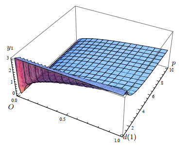
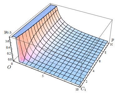
In this paper, a family of potential wells are introduced by means of the modified depths of the potential wells. These potential wells are employed to study the initial-boundary value problem for a wave equation. The expression of the depths of the potential wells is derived. Global existence and finite time blow-up of weak solutions with the subcritical initial energy and the critical initial energy are obtained, respectively. Moreover, some numerical simulations of the depths of the potential wells are carried out.
- Wave equations,
- global existence,
- blow-up,
- potential wells
Citation: Yang Liu, Wenke Li. A family of potential wells for a wave equation[J]. Electronic Research Archive, 2020, 28(2): 807-820. doi: 10.3934/era.2020041

Related Papers:

Abstract

In this paper, a family of potential wells are introduced by means of the modified depths of the potential wells. These potential wells are employed to study the initial-boundary value problem for a wave equation. The expression of the depths of the potential wells is derived. Global existence and finite time blow-up of weak solutions with the subcritical initial energy and the critical initial energy are obtained, respectively. Moreover, some numerical simulations of the depths of the potential wells are carried out.

References

[1]	Standing and travelling waves in a parabolic-hyperbolic system. Discrete Contin. Dyn. Syst. (2019) 39: 5603-5635.
[2]	Qualitative analysis of a nonlinear wave equation. Discrete Contin. Dyn. Syst. (2004) 10: 787-804.
[3]	Global solutions and finite time blow up for damped semilinear wave equations. Ann. Inst. H. Poincaré Anal. Non Linéaire (2006) 23: 185-207.
[4]	Some remarks on the wave equations with nonlinear damping and source terms. Nonlinear Anal. (1996) 27: 1165-1175.
[5]	The method of energy channels for nonlinear wave equations. Discrete Contin. Dyn. Syst. (2019) 39: 6979-6993.
[6]	Global well-posedness of nonlinear wave equation with weak and strong damping terms and logarithmic source term. Adv. Nonlinear Anal. (2020) 9: 613-632.
[7]	J.-L. Lions, Quelques Méthodes de Résolution des Problémes aux Limites non Linéaires, Dunod, Paris, 1969.
[8]	On potential wells and vacuum isolating of solutions for semilinear wave equations. J. Differential Equations (2003) 192: 155-169.
[9]	Global existence for semilinear damped wave equations in relation with the Strauss conjecture. Discrete Contin. Dyn. Syst. (2020) 40: 709-724.
[10]	Wave equations and reaction-diffusion equations with several nonlinear source terms of different sign. Discrete Contin. Dyn. Syst. Ser. B (2007) 7: 171-189.
[11]	Global existence and blow up of solutions for Cauchy problem of generalized Boussinesq equation. Phys. D (2008) 237: 721-731.
[12]	On potential wells and applications to semilinear hyperbolic equations and parabolic equations. Nonlinear Anal. (2006) 64: 2665-2687.
[13]	Existence of global solutions to the Cauchy problem for the semilinear dissipative wave equations. Math. Z. (1993) 214: 325-342.
[14]	Sadle points and instability of nonlinear hyperbolic equations. Israel J. Math. (1975) 22: 273-303.
[15]	On global solution of nonlinear hyperbolic equations. Arch. Rational Mech. Anal. (1968) 30: 148-172.
[16]	Stable and unstable sets for the Cauchy problem for a nonlinear wave equation with nonlinear damping and source terms. J. Math. Anal. Appl. (1999) 239: 213-226.
[17]	Global solution for a generalized Boussinesq equation. Appl. Math. Comput. (2008) 204: 130-136.
[18]	R. Xu, Y. Chen, Y. Yang, S. Chen, J. Shen, T. Yu and Z. Xu, Global well-posedness of semilinear hyperbolic equations, parabolic equations and Schrödinger equations, Electron, J. Differential Equations, 2018 (2018), Paper No. 55, 52 pp.
[19]	Global well-posedness of coupled parabolic systems. Sci. China Math. (2020) 63: 321-356.
[20]	Global existence and finite time blow-up for a class of semilinear pseudo-parabolic equations. J. Funct. Anal. (2013) 264: 2732-2763.
[21]	Global existence and asymptotic behaviour of solutions for a class of fourth order strongly damped nonlinear wave equations. Quart. Appl. Math. (2013) 71: 401-415.
[22]	The initial-boundary value problems for a class of six order nonlinear wave equation. Discrete Contin. Dyn. Syst. (2017) 37: 5631-5649.

Reader Comments

Your name:*

Email:*
© 2020 the Author(s), licensee AIMS Press. This is an open access article distributed under the terms of the Creative Commons Attribution License (http://creativecommons.org/licenses/by/4.0)