Determination of transmission reliability margin for brownout

Awatif Nadia; Md. Sanwar Hossain; Md. Mehedi Hasan; Sinthia Afrin; Md Shafiullah; Md. Biplob Hossain; Khondoker Ziaul Islam; Awatif Nadia; Md. Sanwar Hossain; Md. Mehedi Hasan; Sinthia Afrin; Md Shafiullah; Md. Biplob Hossain; Khondoker Ziaul Islam

doi:10.3934/energy.2021046

AIMS Energy

2021, Volume 9, Issue 5: 1009-1026. doi: 10.3934/energy.2021046

Previous Article Next Article

Research article Special Issues

Determination of transmission reliability margin for brownout

1.
Department of Electrical, Electronic & Communication Engineering, Military Institute of Science and Technology, Dhaka-1216, Bangladesh
2.
Department of Electrical and Electronic Engineering, Bangladesh University of Business and Technology, Dhaka-1216, Bangladesh
3.
Department of Electrical and Electronic Engineering, Green University of Bangladesh, Dhaka-1216, Bangladesh
4.
Interdisciplinary Research Center for Renewable Energy and Power Systems, King Fahd University of Petroleum & Minerals, Dhahran 31261, Saudi Arabia
5.
Department of Electrical and Electronic Engineering, Jashore University of Science and Technology, Jashore-7408, Bangladesh
6.
Information Technology, Murdoch University, 90 South Street, Murdoch, WA 6150, Australia

Received: 23 May 2021 Accepted: 25 August 2021 Published: 02 September 2021

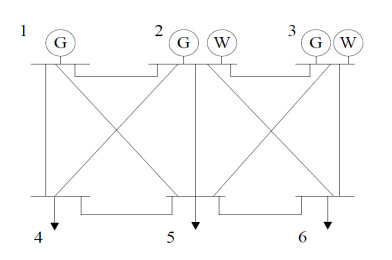
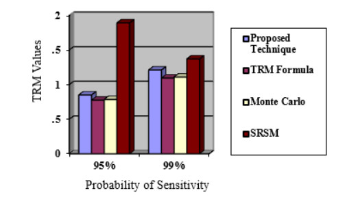
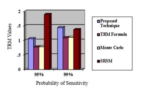
Power shortage is a severe problem in developing countries that are rolling to blackout, but today smart grids have the scope to avoid entire blackouts by transforming them into brownouts. A brownout is an under-voltage condition where the AC supply drops below the nominal value (120 V or 220 V) by about 10%. In a power system network, power shortages or disturbances can occur at any time, and the reliability margin analysis is essential to maintain the stability of the system. Transmission reliability margin (TRM) is a margin that keeps the network secure during any occurrence of disturbance. This paper presents a new approach to compute TRM in the case of brownout. The detailed assessment of TRM largely depends on the estimation of the available transfer power (ATC). In this method, the ATC of the system is calculated considering the effect of alternating current (AC) and direct current (DC) reactive power (Q) flow (DCQF). The entire procedure is carried out for the multi-transaction IEEE-6 bus system, and the results are compared to the current efficiency justification method. Numerical results demonstrate that the proposed technique is an effective alternative for calculating the TRM and is valid compared to the existing technique.
- transmission reliability margin,
- available transfer capability,
- brownout,
- sensitivity of ATC (SATC),
- gamma distribution
Citation: Awatif Nadia, Md. Sanwar Hossain, Md. Mehedi Hasan, Sinthia Afrin, Md Shafiullah, Md. Biplob Hossain, Khondoker Ziaul Islam. Determination of transmission reliability margin for brownout[J]. AIMS Energy, 2021, 9(5): 1009-1026. doi: 10.3934/energy.2021046

Related Papers:

Abstract

Power shortage is a severe problem in developing countries that are rolling to blackout, but today smart grids have the scope to avoid entire blackouts by transforming them into brownouts. A brownout is an under-voltage condition where the AC supply drops below the nominal value (120 V or 220 V) by about 10%. In a power system network, power shortages or disturbances can occur at any time, and the reliability margin analysis is essential to maintain the stability of the system. Transmission reliability margin (TRM) is a margin that keeps the network secure during any occurrence of disturbance. This paper presents a new approach to compute TRM in the case of brownout. The detailed assessment of TRM largely depends on the estimation of the available transfer power (ATC). In this method, the ATC of the system is calculated considering the effect of alternating current (AC) and direct current (DC) reactive power (Q) flow (DCQF). The entire procedure is carried out for the multi-transaction IEEE-6 bus system, and the results are compared to the current efficiency justification method. Numerical results demonstrate that the proposed technique is an effective alternative for calculating the TRM and is valid compared to the existing technique.

References

[1]	Billinton R (1994) Evaluation of reliability worth in an electric power system. Reliab Eng Syst Saf 46: 15-23. doi: 10.1016/0951-8320(94)90044-2
[2]	Bazovsky I (2004) Reliability Theory and Practice. Dover Publications Inc., New York, USA.
[3]	Sun X, Chen J, Zhu Q, et al. (2016) Assessment of transmission reliability margin using stochastic response surface method. IEEE Power and Energy Society General Meeting (PESGM).
[4]	Zhang J, Dobson I, Alvarado FL (2004) Quantifying transmission reliability margin. Int J Electr Power Energy Syst 26: 697-702. doi: 10.1016/S0142-0615(04)00071-7
[5]	Rodrigues AB, Silva MG Da (2011) Chronological simulation for transmission reliability margin evaluation with time-varying loads. Int J Electr Power Energy Syst 33: 1054-1061. doi: 10.1016/j.ijepes.2011.01.024
[6]	Othman MM bin, Mohamed A, Hussain A (2008) Determination of transmission reliability margin using parametric bootstrap technique. IEEE Trans Power Syst 23: 1689-1700. doi: 10.1109/TPWRS.2008.2004734
[7]	Zaini RH, Othman MM bin, Musirin I, et al. (2010) Determination of transmission reliability margin considering uncertainties of system operating condition and transmission line outage. Eur Trans Electr Power 21: 380-397. doi: 10.1002/etep.448
[8]	Li D, Chen Y, Lu W, et al. (2011) Stochastic response surface method for reliability analysis of rock slopes involving correlated non-normal variables. Comput Geotech 38: 58-68. doi: 10.1016/j.compgeo.2010.10.006
[9]	Nadia A, Chowdhury AH (2019) Transmission reliability margin calculation by modified DC load flow method. International Conference on Advances in Electrical Engineering (ICAEE).
[10]	Othman MM bin, Mohamed A, Hussain A (2006) Determination of available transfer capability incorporating transmission reliability margin. IEEE International Power and Energy Conference.
[11]	Khatavkar V, Swathi D, Mayadeo H, et al. (2018) Short-term estimation of transmission reliability margin using artificial neural networks. In International Proceedings on Advances in Soft Computing, Intelligent Systems and Applications, Springer, Singapore.
[12]	Nadia A, Chowdhury AH, Mahfuj E, et al. (2020) Determination of transmission reliability margin using AC load flow. AIMS Energy 8: 701-720. doi: 10.3934/energy.2020.4.701
[13]	Ou Y, Singh C (2002) Assessment of available transfer capability and margins. IEEE Trans Power Syst 17: 463-468. doi: 10.1109/TPWRS.2002.1007919
[14]	Ian D, Greene S, Rajaraman R, et al. (2001) Electric power transfer capability: concepts, applications, sensitivity, and uncertainty. PSERC: 01-34.
[15]	Sharma AK, Kumar J (2011) ACPTDF for Multi-transactions and ATC determination in deregulated markets. Inter J Electr Comput Eng (IJECE) 1: 71-84.
[16]	Manjusha S, Rao JS (2015) Determination of ATC for single and multiple transactions in restructured power systems. Int J Electr Electr Eng, 2.
[17]	Kumar A, Kumar M (2013) Available transfer capability determination using power transfer distribution factors. Int J Emerging Electr Power Syst 3: 1171-1176.
[18]	Duong TL, Nguyen TT, Nguyen NA, et al. (2020) Available transfer capability determination for the electricity market using cuckoo search algorithm. Eng Technol Appl Sci Res10: 5340-5345. doi: 10.48084/etasr.3338
[19]	Chen H, Fang X, Zhang R, et al. (2017) Available transfer capability evaluation in a deregulated electricity market considering correlated wind power. IET Gener, Trans Distrib 12: 53-61. doi: 10.1049/iet-gtd.2016.1883
[20]	Ahmad AS, Adamu SS, Buhari M (2019) Available transfer capability enhancement with FACTS using hybrid PI-PSO. Turk J Electr Eng Comput Sci 27: 2881-2897. doi: 10.3906/elk-1812-54
[21]	Mohammed OO, Mustafa MW, Mohammed DSS, et al. (2019) Available transfer capability calculation methods: A comprehensive review. Int Trans Electr Energy Syst 29: 1-24. doi: 10.1002/2050-7038.2846
[22]	Grijalva S, Sauer PW (1999) Reactive power considerations in linear ATC computation. Proceedings of the 32nd Annual Hawaii International Conference on Systems Sciences. HICSS-32.
[23]	Gao Y, Li G, Zhou M (2009) Available transfer capability evaluation based on sensitivity analysis. IFAC Proceedings Vol 42: 62-67. doi: 10.3182/20090705-4-SF-2005.00013
[24]	Christie RD, Wollenberg BF, Wangensteen I (2000) Transmission management in the deregulated environment. Proceedings IEEE 88: 170-195. doi: 10.1109/5.823997
[25]	Beagam KSH, Jayashree R, Khan MA (2017) A new DC power flow model for Q flow analysis for use in reactive power market. Eng Sci Technol, Int J 20: 721-729.
[26]	Greene S, Dobson I, Alvarado FL (2002) Sensitivity of transfer capability margins with a fast formula. IEEE Trans Power Syst 17: 34-40. doi: 10.1109/59.982190
[27]	Nadia A, Chowdhury AH (2019) Correlation between transmission reliability margin and standard deviation of uncertainty. 5th International Conference on Advances in Electrical Engineering (ICAEE).
[28]	Lane JE, Zulim D (2011) Equipment and methods for emergency lighting that provides brownout detection and protection. ABL IP Holding LLC, U.S. Patent 7,863,832.
[29]	Basina DR, Kumar S, Padhi S, et al. (2020) Brownout based blackout avoidance strategies in smart grids. IEEE Trans Sustainable Comput.
[30]	Zhang Y, Wang L, Xiang Y, et al. (2015) Power system reliability evaluation with SCADA cybersecurity considerations. IEEE Trans Smart Grid 6: 1707-1721. doi: 10.1109/TSG.2015.2396994
[31]	Nadia A, Hossain MS, Hasan MM, et al. (2021) Quantifying TRM by modified DCQ load flow method. Eur J Electr Eng 23: 157-163. doi: 10.18280/ejee.230210
[32]	Hossain MS, Rahman MF (2020) Hybrid solar PV/Biomass powered energy efficient remote cellular base stations. Int J Renewable Energy Res 10: 329-342.
[33]	Jahid A, Hossain MS, Monju MKH, et al. (2020) Techno-Economic and energy efficiency analysis of optimal power supply solutions for green cellular base stations. IEEE Access 8: 43776-43795. doi: 10.1109/ACCESS.2020.2973130
[34]	Hossain MS, Jahid A, Islam KZ, et al. (2020) Solar PV and biomass resources-based sustainable energy supply for Off-Grid cellular base stations. IEEE Access 8: 53817-53840. doi: 10.1109/ACCESS.2020.2978121
[35]	Hossain MS, Jahid A, Islam KZ, et al. (2020) Multi-Objective optimum design of hybrid renewable energy system for sustainable energy supply to a green cellular networks. Sustainability 12: 3536. doi: 10.3390/su12093536
[36]	Abunima H, Teh J, Lai CM, et al. (2018) A systematic review of reliability studies on composite power systems: a coherent taxonomy motivation, open challenges, recommendations, and new research directions. Energies 11: 2417. doi: 10.3390/en11092417
[37]	Paveethra SR, Kalavalli C, Vijayalakshmi S, et al. (2020) Evaluation of voltage stability of transmission line with contingency analysis. Int J Sci Technol Res 9: 1-4.
[38]	Li X, Jiang T, Liu G, et al. (2020) Bootstrap-based confidence interval estimation for thermal security region of bulk power grid. Int J Electr Power Energy Syst 115: 105498. doi: 10.1016/j.ijepes.2019.105498
[39]	Adusumilli BS, Kumar BK (2018) Modified affine arithmetic based continuation power flow analysis for voltage stability assessment under uncertainty. IET Gener, Trans Distrib 12: 4225-4232. doi: 10.1049/iet-gtd.2018.5479
[40]	Lee Y, Song H (2019) A reactive power compensation strategy for voltage stability challenges in the Korean power system with dynamic loads. Sustainability 11: 326. doi: 10.3390/su11020326
[41]	Teh J, Lai CM, Cheng YH (2017) Impact of the real-time thermal loading on the bulk electric system reliability. IEEE Trans Reliab 66: 1110-1119. doi: 10.1109/TR.2017.2740158
[42]	Teh J (2018) Uncertainty analysis of transmission line end-of-life failure model for bulk electric system reliability studies. IEEE Trans Reliab 67: 1261-1268. doi: 10.1109/TR.2018.2837114
[43]	Teh J, Lai CM (2019) Reliability impacts of the dynamic thermal rating system on smart grids considering wireless communications. IEEE Access 7: 41625-41635. doi: 10.1109/ACCESS.2019.2907980
[44]	Teh J, Lai CM (2019) Reliability impacts of the dynamic thermal rating and battery energy storage systems on wind-integrated power networks. Sustainable Energy, Grids Networks 20: 100268. doi: 10.1016/j.segan.2019.100268
[45]	Metwaly MK, Teh J (2020) Probabilistic peak demand matching by battery energy storage alongside dynamic thermal ratings and demand response for enhanced network reliability. IEEE Access 8: 181547-181559. doi: 10.1109/ACCESS.2020.3024846
[46]	Teh J, Lai CM, Cheng YH (2018) Improving the penetration of wind power with dynamic thermal rating system, static VAR compensator and multi-objective genetic algorithm. Energies 11: 815. doi: 10.3390/en11040815
[47]	Metwaly MK, Teh J (2020) Optimum network ageing and battery sizing for improved wind penetration and reliability. IEEE Access 8: 118603-118611. doi: 10.1109/ACCESS.2020.3005676
[48]	Hossain MS, Rahman M, Sarker MT, et al. (2019) A smart IoT based system for monitoring and controlling the sub-station equipment. Internet of Things 7: 100085. doi: 10.1016/j.iot.2019.100085
[49]	Jahid A, Islam KZ, Hossain S, et al. (2019) Performance evaluation of cloud radio access network with hybrid power supplies. In Proceedings of the International Conference on Sustainable Technologies for Industry 4.0 (STI).
[50]	Haque ME, Asikuzzaman M, Khan IU, et al. (2020) Comparative study of IoT-based topology maintenance protocol in a wireless sensor network for structural health monitoring. Remote Sensing 12: 2358. doi: 10.3390/rs12152358
[51]	Sauer PW (1997) Technical challenges of computing available transfer capability (ATC) in electric power systems. In Proceedings of the Thirtieth Hawaii International Conference on System Sciences 5: 589-593. doi: 10.1109/HICSS.1997.663220
[52]	Sauer PW (1998) Alternatives for calculating transmission reliability margin (TRM) in available transfer capability (ATC). In Proceedings of the Thirty-First Hawaii International Conference on System Sciences 3: 89. doi: 10.1109/HICSS.1998.656069

Reader Comments

Your name:*

Email:*
© 2021 the Author(s), licensee AIMS Press. This is an open access article distributed under the terms of the Creative Commons Attribution License (http://creativecommons.org/licenses/by/4.0)