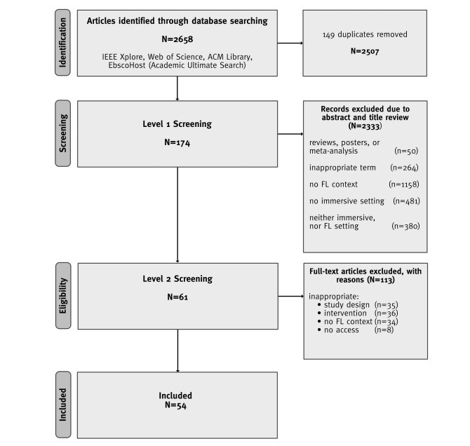
This study provides a systematic literature review of research (2001–2020) in the field of teaching and learning a foreign language and intercultural learning using immersive technologies. Based on 2507 sources, 54 articles were selected according to a predefined selection criteria. The review is aimed at providing information about which immersive interventions are being used for foreign language learning and teaching and where potential research gaps exist. The papers were analyzed and coded according to the following categories: (1) investigation form and education level, (2) degree of immersion, and technology used, (3) predictors, and (4) criterions. The review identified key research findings relating the use of immersive technologies for learning and teaching a foreign language and intercultural learning at cognitive, affective, and conative levels. The findings revealed research gaps in the area of teachers as a target group, and virtual reality (VR) as a fully immersive intervention form. Furthermore, the studies reviewed rarely examined behavior, and implicit measurements related to inter- and trans-cultural learning and teaching. Inter- and transcultural learning and teaching especially is an underrepresented investigation subject. Finally, concrete suggestions for future research are given. The systematic review contributes to the challenge of interdisciplinary cooperation between pedagogy, foreign language didactics, and Human-Computer Interaction to achieve innovative teaching-learning formats and a successful digital transformation.
Citation: Rebecca M. Hein, Carolin Wienrich, Marc E. Latoschik. A systematic review of foreign language learning with immersive technologies (2001-2020)[J]. AIMS Electronics and Electrical Engineering, 2021, 5(2): 117-145. doi: 10.3934/electreng.2021007
This study provides a systematic literature review of research (2001–2020) in the field of teaching and learning a foreign language and intercultural learning using immersive technologies. Based on 2507 sources, 54 articles were selected according to a predefined selection criteria. The review is aimed at providing information about which immersive interventions are being used for foreign language learning and teaching and where potential research gaps exist. The papers were analyzed and coded according to the following categories: (1) investigation form and education level, (2) degree of immersion, and technology used, (3) predictors, and (4) criterions. The review identified key research findings relating the use of immersive technologies for learning and teaching a foreign language and intercultural learning at cognitive, affective, and conative levels. The findings revealed research gaps in the area of teachers as a target group, and virtual reality (VR) as a fully immersive intervention form. Furthermore, the studies reviewed rarely examined behavior, and implicit measurements related to inter- and trans-cultural learning and teaching. Inter- and transcultural learning and teaching especially is an underrepresented investigation subject. Finally, concrete suggestions for future research are given. The systematic review contributes to the challenge of interdisciplinary cooperation between pedagogy, foreign language didactics, and Human-Computer Interaction to achieve innovative teaching-learning formats and a successful digital transformation.

| [1] |
Ahn SJ, Bostick J, Ogle E, et al. (2016) Experiencing nature: Embodying animals in immersive virtual environments increases inclusion of nature in self and involvement with nature. Journal of Computer-Mediated Communication 21: 399–419. doi: 10.1111/jcc4.12173

|
| [2] |
Banakou D, Groten R, Slater M (2013) Illusory ownership of a virtual child body causes overestimation of object sizes and implicit attitude changes. Proceedings of the National Academy of Sciences 110: 12846–12851. doi: 10.1073/pnas.1306779110
|
| [3] | Barreira J, Bessa M, Pereira LC, et al. (2012) MOW: Augmented Reality game to learn words in different languages: Case study: Learning English names of animals in elementary school. In 7th Iberian conference on information systems and technologies (CISTI 2012). 1–6. IEEE. |
| [4] | Barrett MD (2011) Intercultural competence. EWC Statement Series 2: 23–27. |
| [5] | Bazzaza MW, Alzubaidi M, Zemerly MJ, et al. (2016) Impact of smart immersive mobile learning in language literacy education. In 2016 IEEE Global Engineering Education Conference (EDUCON). 443–447. IEEE. |
| [6] | Berns A, Mota JM, Ruiz-Rube I, et al. (2018) Exploring the potential of a 360 video application for foreign language learning. In Proceedings of the Sixth International Conference on Technological Ecosystems for Enhancing Multiculturality. 776–780. |
| [7] | Blell G, Doff S (2014) Mehrsprachigkeit und Mehrkulturalität: Einführung in das Thema. Zeitschrift für Interkulturellen Fremdsprachenunterricht 19. |
| [8] |
Bond M, Marín VI, Dolch C, et al. (2018) Digital transformation in German higher education: student and teacher perceptions and usage of digital media. Int J Educ Technol H 15: 1–20. doi: 10.1186/s41239-017-0083-9
|
| [9] |
Buhl H, Winter R (2009) Full virtualization – BISE's contribution to a vision. Business and Information Systems Engineering 1: 133–136. doi: 10.1007/s12599-008-0023-2
|
| [10] | Byram M, Doyé P (1999) Intercultural competence and foreign language learning in the primary school. The teaching of modern foreign languages in the primary school, 138–151. |
| [11] | Chabot S, Drozdal J, Peveler M, et al. (2020) A collaborative, immersive language learning environment using augmented panoramic imagery. In 2020 6th International Conference of the Immersive Learning Research Network (iLRN), 225–229. |
| [12] | Chang YJ, Chen CH, Huang WT, et al. (2011) Investigating students' perceived satisfaction, behavioral intention, and effectiveness of English learning using augmented reality. In 2011 IEEE International Conference on Multimedia and Expo. 1–6. |
| [13] | Chen G, Starosta W (1999) A review of the concept of intercultural awareness. Human Communication 2: 27–54. |
| [14] | Chen CP, Wang CH (2015) The effects of learning style on mobile augmented-reality-facilitated English vocabulary learning. In 2015 2nd International Conference on Information Science and Security (ICISS). 1–4. |
| [15] |
Chen YL (2016) The effects of virtual reality learning environment on student cognitive and linguistic development. The Asia-Pacific Education Researcher 25: 637–646. doi: 10.1007/s40299-016-0293-2
|
| [16] | Chen SY, Hung CY, Chang YC, et al. (2018) A study on integrating augmented reality technology and game-based learning model to improve motivation and effectiveness of learning English vocabulary. In 2018 1st International Cognitive Cities Conference (IC3). 24–27. |
| [17] | Chen MP, Wang LC, Zou D, et al. (2020) Effects of captions and English proficiency on learning effectiveness, motivation and attitude in augmented-reality-enhanced theme-based contextualized EFL learning. Computer Assisted Language Learning, 1–31. |
| [18] | Chen MRA, Hwang GJ (2020) Effects of experiencing authentic contexts on English speaking performances, anxiety and motivation of EFL students with different cognitive styles. Interactive Learning Environments, 1–21. |
| [19] |
Chen Y, Smith TJ, York CS, et al. (2020) Google Earth Virtual Reality and expository writing for young English Learners from a Funds of Knowledge perspective. Computer Assisted Language Learning 33: 1–25. doi: 10.1080/09588221.2018.1544151
|
| [20] |
Chen CH (2020) AR videos as scaffolding to foster students' learning achievements and motivation in EFL learning. British Journal of Educational Technology 51: 657–672. doi: 10.1111/bjet.12902
|
| [21] | Chew SW, Jhu JY, Chen NS (2018) The effect of learning English idioms using scaffolding strategy through situated learning supported by augmented reality. In 2018 IEEE 18th International Conference on Advanced Learning Technologies (ICALT). 390–394. |
| [22] | Chung LY (2011) Using avatars to enhance active learning: Integration of virtual reality tools into college English curriculum. In The 16th North-East Asia Symposium on Nano, Information Technology and Reliability. 29–33. |
| [23] | Chung LY (2012) Virtual Reality in college English curriculum: Case study of integrating second life in freshman English course. In 2012 26th International Conference on Advanced Information Networking and Applications Workshops. 250–253. |
| [24] |
Cooper C, Varley-Campbell J, Booth A, et al. (2018) Systematic review identifies six metrics and one method for assessing literature search effectiveness but no consensus on appropriate use. J clin epidemiol 99: 53–63. doi: 10.1016/j.jclinepi.2018.02.025
|
| [25] |
Cornillie F, Clarebout G, Desmet P (2012) Between learning and playing? Exploring learners' perceptions of corrective feedback in an immersive game for English pragmatics. ReCALL: Journal of Eurocall 24: 257–278. doi: 10.1017/S0958344012000146
|
| [26] | Dalim CSC, Dey A, Piumsomboon T, et al. (2016) TeachAR: An interactive augmented reality tool for teaching basic English to non-native children. In 2016 IEEE International Symposium on Mixed and Augmented Reality (ISMAR-Adjunct). 82–86. |
| [27] | De Freitas S (2006) Learning in immersive worlds: A review of game-based learning. 2–60. |
| [28] | De Grove F, Van Looy J, Courtois C (2010) Towards a serious game experience model: Validation, extension and adaptation of the GEQ for use in an educational context. In Playability and player experience. 10: 47–61. Breda University of Applied Sciences. |
| [29] | Draxler F, Labrie A, Schmidt A, et al. (2020) Augmented reality to enable users in learning case grammar from their real-world interactions. In Proceedings of the 2020 CHI Conference on Human Factors in Computing Systems. 1–12. |
| [30] |
Eisenmann M, Grimm N, Volkmann L (2010) 92. Teaching the new English cultures and literatures. English and American Studies in German 2009: 164–166. doi: 10.1515/9783484431225.164
|
| [31] | Eisenmann M (2019) Teaching English: Differentiation and Individualisation. utb GmbH. |
| [32] |
Fast-Berglund Å, Gong LL (2018) Testing and validating extended reality (xR) technologies in manufacturing. Procedia Manuf 25: 31–38. doi: 10.1016/j.promfg.2018.06.054
|
| [33] |
Fernández SS, Pozzo MI (2017) Intercultural competence in synchronous communication between native and non-native speakers of Spanish. Language Learning in Higher Education 7: 109–135. doi: 10.1515/cercles-2017-0003
|
| [34] |
Garzon J, Acevedo J (2019) Meta-analysis of the impact of Augmented Reality on students' learning gains. Educational Research Review 27: 244–260. doi: 10.1016/j.edurev.2019.04.001
|
| [35] | Gelsomini M, Leonardi G, Garzotto F (2020) Embodied learning in immersive smart spaces. In Proceedings of the 2020 CHI Conference on Human Factors in Computing Systems. 1–14. |
| [36] | Giraudeau P, Olry A, Roo JS, et al. (2019) CARDS: a mixed-reality system for collaborative learning at school. In Proceedings of the 2019 ACM International Conference on Interactive Surfaces and Spaces. 55–64. |
| [37] | Grünewald A (2016) Üben und Übungen im Fremdsprachenunterricht. Üben und Übungen beim Fremdsprachenlernen: Perspektiven und Konzepte für Unterricht und Forschung. Arbeitspapiere der 36. Frühjahrskonferenz zur Erforschung des Fremdsprachenunterrichts, 84. |
| [38] | Guillén-Nieto V, Aleson-Carbonell M (2012) Serious games and learning effectiveness: The case of It'sa Deal! Computers and Education 58: 435–448. |
| [39] |
Hamilton D, McKechnie J, Edgerton E (2020) Immersive virtual reality as a pedagogical tool in education: a systematic literature review of quantitative learning outcomes and experimental design. Journal of Computer Education 8: 1–32. doi: 10.1007/s40692-020-00169-2
|
| [40] | Hammer M (2012) The intercultural development inventory: A new frontier in assessment and development of intercultural competence. Sterling, VA: Stylus Publishing. In M. Vande Berg, R. M. Paige, and K. H. Lou (Eds.). Student learning abroad, 115–136. |
| [41] | Hao KC, Lee LC (2019) The development and evaluation of an educational game integrating augmented reality, ARCS model, and types of games for English experiment learning: an analysis of learning. Interactive Learning Environments, 1–14. |
| [42] |
Hassani K, Nahvi A, Ahmadi A (2016) Design and implementation of an intelligent virtual environment for improving speaking and listening skills. Interactive Learning Environments 24: 252–271. doi: 10.1080/10494820.2013.846265
|
| [43] | He J, Ren J, Zhu G, et al. (2014) Mobile-based AR application helps to promote EFL children's vocabulary study. In 2014 IEEE 14th International Conference on Advanced Learning Technologies. 431–433. |
| [44] |
Herrera F, Bailenson J, Weisz E, et al. (2018) Building long-term empathy: A large-scale comparison of traditional and virtual reality perspective-taking. PLOS ONE 13: e0204494. doi: 10.1371/journal.pone.0204494
|
| [45] | Ho SC, Hsieh SW, Sun PC, et al. (2017) To activate English learning: Listen and speak in real life context with an AR featured u-learning system. Journal of Educational Technology and Society 20: 176–187. |
| [46] | Hsieh M (2016) Development and evaluation of a mobile AR assisted learning system for English learning. 2016 International Conference on Applied System Innovation (ICASI), Okinawa, 1-4. |
| [47] | Hsieh MC (2016) Teachers' and students' perceptions toward augmented reality materials. In 2016 5th IIAI International Congress on Advanced Applied Informatics (IIAI-AAI). 1180–1181. |
| [48] |
Hsu TC (2019) Effects of gender and different augmented reality learning systems on English vocabulary learning of elementary school students. Universal Access in the Information Society 18: 315–325. doi: 10.1007/s10209-017-0593-1
|
| [49] | Huang X, Han G, He J, et al. (2018) Design and Application of a VR English Learning Game Based on the APT Model. In 2018 Seventh International Conference of Educational Innovation through Technology (EITT). 68–72. |
| [50] |
Hung HC, Young SSC (2015) An investigation of game-embedded handheld devices to enhance English learning. Journal of Educational Computing Research 52: 548–567. doi: 10.1177/0735633115571922
|
| [51] |
Ibrahim A, Huynh B, Downey J, et al. (2018) Arbis pictus: A study of vocabulary learning with augmented reality. IEEE T Vis Comput Gr 24: 2867–2874. doi: 10.1109/TVCG.2018.2868568
|
| [52] | Ji S, Li K, Zou L (2019) The Effect of 360-Degree Video Authentic Materials on EFL Learners' Listening Comprehension. In 2019 International Joint Conference on Information, Media and Engineering (IJCIME). 288–293. |
| [53] |
Johnson-Glenberg MC, Birchfield DA, Tolentino L, et al. (2014) Collaborative embodied learning in mixed reality motion-capture environments: Two science studies. Journal of Educational Psychology 106: 86. doi: 10.1037/a0034008
|
| [54] | Khatoony S (2019) An Innovative Teaching with Serious Games through Virtual Reality Assisted Language Learning. In 2019 International Serious Games Symposium (ISGS). 100–108. |
| [55] | Kincheloe Joe L (2008) Critical Pedagogy Primer 2nd edition. English: New York, NY: Peter Lang. |
| [56] | Küçük S, Yylmaz RM, Göktap Y (2014) Augmented reality for learning English: Achievement, attitude and cognitive load levels of students. Education and Science/Egitim ve Bilim 39. |
| [57] | Küster L (2014) Zur Einführung in den Themenschwerpunkt. Fremdsprachen lehren und lernen 43: 2. |
| [58] | Lan YJ (2015) Contextual EFL learning in a 3D virtual environment. Language Learning and Technology 19: 16–31. |
| [59] |
Lee K, Kweon SO, Lee S, et al. (2014) POSTECH immersive English study (POMY): Dialog-based language learning game. IEICE T Inf Syst 97: 1830–1841. doi: 10.1587/transinf.E97.D.1830
|
| [60] |
Lee SM, Park M (2020) Reconceptualization of the context in language learning with a location-based AR app. Computer Assisted Language Learning 33: 936–959. doi: 10.1080/09588221.2019.1602545
|
| [61] | Leyva F, Plummer CJ (2015) National Institute for Health and Care Excellence 2014 guidance on cardiac implantable electronic devices: health economics reloaded. |
| [62] | Li KC, Tsai CW, Chen CT, et al. (2015) The design of immersive English learning environment using augmented reality. In 2015 8th International Conference on Ubi-Media Computing (UMEDIA). 174-179. |
| [63] | Liaw ML (2019) EFL learners' intercultural communication in an open social virtual environment. Journal of Educational Technology and Society 22: 38–55. |
| [64] |
Liou HC (2012) The roles of Second Life in a college computer-assisted language learning (CALL) course in Taiwan, ROC. Computer Assisted Language Learning 25: 365–382. doi: 10.1080/09588221.2011.597766
|
| [65] |
Liu IF, Chen MC, Sun YS, et al. (2010) Extending the TAM model to explore the factors that affect intention to use an online learning community. Computers and education 54: 600–610. doi: 10.1016/j.compedu.2009.09.009
|
| [66] | Liu E, Liu C, Yang Y, et al. (2018) Design and implementation of an augmented reality application with an English Learning Lesson. In 2018 IEEE International Conference on Teaching, Assessment, and Learning for Engineering (TALE) 494–499. |
| [67] | Lorenzo CM, Lezcano L, Alonso SS (2013) Language Learning in Educational Virtual Worlds-a TAM Based Assessment. J UCS 19: 1615–1637. |
| [68] | Matveev AV (2002) The perception of intercultural communication competence by American and Russian managers with experience on multicultural teams (Doctoral dissertation, Ohio University). |
| [69] | Milgram P, Kishino F (1994) A taxonomy of mixed reality visual displays. IEICE T Inf Syst 77: 1321–1329. |
| [70] |
Moher D, Liberati A, Tetzlaff J, et al. (2011) Bevorzugte Report Items für systematische Übersichten und Meta-Analysen: Das PRISMA-Statement. DMW-Deutsche Medizinische Wochenschrift 136: e9–e15. doi: 10.1055/s-0031-1272982
|
| [71] |
Neumeier P (2005) A closer look at blended learning–parameters for designing a blended learning environment for language teaching and learning. ReCALL: the Journal of EUROCALL 17: 163. doi: 10.1017/S0958344005000224
|
| [72] |
Oberdörfer S, Latoschik ME (2019) Predicting learning effects of computer games using the Gamified Knowledge Encoding Model. Entertain Comput 32: 100315. doi: 10.1016/j.entcom.2019.100315
|
| [73] | Oberdörfer S, Elsässer A, Schraudt D, et al. (2020) Horst-The teaching frog: learning the anatomy of a frog using tangible AR. In Proceedings of the Conference on Mensch und Computer. 303–307. |
| [74] |
Peck T, Seinfeld S, Aglioti S, et al. (2013) Putting yourself in the skin of a black avatar reduces implicit racial bias. Consciousness and cognition 22: 779–787. doi: 10.1016/j.concog.2013.04.016
|
| [75] |
Qu C, Ling Y, Heynderickx I, et al. (2015) Virtual bystanders in a language lesson: examining the effect of social evaluation, vicarious experience, cognitive consistency and praising on students' beliefs, self-efficacy and anxiety in a virtual reality environment. PloS one 10: e0125279. doi: 10.1371/journal.pone.0125279
|
| [76] | Quintín E, Sanz C, Zangara A (2016) The impact of role-playing games through Second Life on the oral practice of linguistic and discursive sub-competences in English. In 2016 International Conference on Collaboration Technologies and Systems (CTS). 148–155. |
| [77] |
Ratan R, Beyea D, Li B, et al. (2020) Avatar characteristics induce 'users' behavioral conformity with small-to-medium effect sizes: A meta-analysis of the proteus effect. Media Psychology 23: 651–675. doi: 10.1080/15213269.2019.1623698
|
| [78] |
Redondo B, Cózar-Gutiérrez R, González-Calero JA, et al. (2020) Integration of augmented reality in the teaching of English as a foreign language in early childhood education. Early Childhood Education Journal 48: 147–155. doi: 10.1007/s10643-019-00999-5
|
| [79] | Ripka G, Grafe S, Latoschik ME (2020) Preservice Teachers' encounter with Social VR–Exploring Virtual Teaching and Learning Processes in Initial Teacher Education. In SITE Interactive Conference. 549–562. Association for the Advancement of Computing in Education (AACE). |
| [80] | Sherman WR, Craig AB (2003) Understanding virtual reality. San Francisco, CA: Morgan Kauffman. |
| [81] | Shih YC, Yang MT (2008) A collaborative virtual environment for situated language learning using VEC3D. Educational Technology and Society 11: 56–68. |
| [82] |
Shih YC (2015) A virtual walk through London: Culture learning through a cultural immersion experience. Computer Assisted Language Learning 28: 407–428. doi: 10.1080/09588221.2013.851703
|
| [83] | Skarbez R, Frederick PB, Mary CW (2018) Immersion and Coherence in a Stressful Virtual Environment. In Proceedings of the 24th Acm Symposium on Virtual Reality Software and Technology. 1–11. |
| [84] |
Slater M, Wilbur S (1997) A framework for immersive virtual environments (FIVE): Speculations on the role of presence in virtual environments. Presence: Teleoperators and Virtual Environments 6: 603–616. doi: 10.1162/pres.1997.6.6.603
|
| [85] |
Slater M (1999) Measuring presence: A response to the Witmer and Singer presence questionnaire. Presence 8: 560–565. doi: 10.1162/105474699566477
|
| [86] | Slater M (2003) A note on presence terminology. Presence connect 3: 1–5. |
| [87] |
Sanchez-Vives MV, Mel S (2005) From presence to consciousness through virtual reality. Nat Rev Neurosci 6: 332–339. doi: 10.1038/nrn1651
|
| [88] |
Slater M (2009) Place illusion and plausibility can lead to realistic behaviour in immersive virtual environments. Philos T R Soc B 364: 3549–3557. doi: 10.1098/rstb.2009.0138
|
| [89] | Tulodziecki G, Grafe S (2012) Approaches to learning with media and media literacy education–trends and current situation in Germany. Journal of Media Literacy Education 4: 5. |
| [90] | Tulodziecki G, Grafe S, Herzig B (2019) Medienbildung in Schule und Unterricht: Grundlagen und Beispiele. UTB GmbH. |
| [91] | Vate-U-Lan P (2012) An augmented reality 3d pop-up book: the development of a multimedia project for English language teaching. In 2012 IEEE International Conference on Multimedia and Expo. 890–895. |
| [92] | Vedadi S, Abdullah ZB, Cheok AD (2019) The Effects of Multi-Sensory Augmented Reality on Students' Motivation in English Language Learning. In 2019 IEEE Global Engineering Education Conference (EDUCON). 1079–1086. |
| [93] |
Wang CX, Calandra B, Hibbard ST, et al. (2012) Learning effects of an experimental EFL program in Second Life. Educational Technology Research and Development 60: 943–961. doi: 10.1007/s11423-012-9259-0
|
| [94] |
Wang YF, Petrina S, Feng F (2017) VILLAGE—V irtual I mmersive L anguage L earning and G aming E nvironment: Immersion and presence. British Journal of Educational Technology 48: 431–450. doi: 10.1111/bjet.12388
|
| [95] |
Wienrich C, Johanna G (2020) AppRaiseVR–An Evaluation Framework for Immersive Experiences. I-Com 19: 103–121. doi: 10.1515/icom-2020-0008
|
| [96] | Wienrich C, Döllinger NI, Hein R (2020) Mind the Gap: A Framework (BehaveFIT) Guiding The Use of Immersive Technologies in Behavior Change Processes. arXiv preprint arXiv: 2012.10912. |
| [97] | Wienrich C, Eisenmann M, Latoschik ME, et al. (2020) CoTeach - Connected Teacher Education. VRinSight Greenpaper 53–55. |
| [98] |
Witmer BG, Singer MJ (1998) Measuring presence in virtual environments: A presence questionnaire. Presence 7: 225–240. doi: 10.1162/105474698565686
|
| [99] |
Wohlgenannt I, Simons A, Stieglitz S (2020) Virtual Reality. Business and Information Systems Engineering 5: 455–461. doi: 10.1007/s12599-020-00658-9
|
| [100] | Wu MH (2019) The applications and effects of learning English through augmented reality: A case study of Pokémon go. Computer Assisted Language Learning, 1–35. |
| [101] |
Yang MT, Liao WC (2014) Computer-assisted culture learning in an online augmented reality environment based on free-hand gesture interaction. IEEE T Learn Technol 7: 107–117. doi: 10.1109/TLT.2014.2307297
|
| [102] | Yeh HC, Tseng SS, Heng L (2020) Enhancing EFL students' intracultural learning through virtual reality. Interactive Learning Environments, 1–10. |
| [103] |
Zhang X, Zhou M (2019) Interventions to promote 'learners' intercultural competence: A meta-analysis. International Journal of Intercultural Relations 71: 31–47. doi: 10.1016/j.ijintrel.2019.04.006
|
Figures(5) / Tables(4)

Rebecca M. Hein, Carolin Wienrich, Marc E. Latoschik. A systematic review of foreign language learning with immersive technologies (2001-2020)[J]. AIMS Electronics and Electrical Engineering, 2021, 5(2): 117-145. doi: 10.3934/electreng.2021007


 DownLoad: