Application of read-across methods as a framework for the estimation of emissions from chemical processes

Sudhakar Takkellapati; Michael A. Gonzalez; Sudhakar Takkellapati; Michael A. Gonzalez

doi:10.3934/ctr.2023018

Clean Technologies and Recycling

2023, Volume 3, Issue 4: 283-300. doi: 10.3934/ctr.2023018

Previous Article Next Article

Research article Topical Sections

Application of read-across methods as a framework for the estimation of emissions from chemical processes

US Environmental Protection Agency, Office of Research and Development, Center for Environmental Solutions and Emergency Response, Land Remediation and Technology Division, Environmental Decision Analytics Branch, 26 W. Martin Luther King Dr., Cincinnati, OH 45268, USA

Received: 13 November 2023 Revised: 19 December 2023 Accepted: 27 December 2023 Published: 28 December 2023

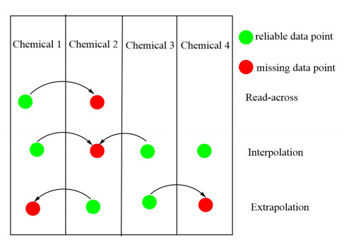
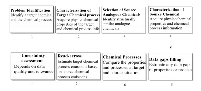
The read-across method is a popular data gap filling technique with developed application for multiple purposes, including regulatory. Within the US Environmental Protection Agency's (US EPA) New Chemicals Program under Toxic Substances Control Act (TSCA), read-across has been widely used, as well as within technical guidance published by the Organization for Economic Co-operation and Development, the European Chemicals Agency, and the European Center for Ecotoxicology and Toxicology of Chemicals for filling chemical toxicity data gaps. Under the TSCA New Chemicals Review Program, US EPA is tasked with reviewing proposed new chemical applications prior to commencing commercial manufacturing within or importing into the United States. The primary goal of this review is to identify any unreasonable human health and environmental risks, arising from environmental releases/emissions during manufacturing and the resulting exposure from these environmental releases. The authors propose the application of read-across techniques for the development and use of a framework for estimating the emissions arising during the chemical manufacturing process. This methodology is to utilize available emissions data from a structurally similar analogue chemical or a group of structurally similar chemicals in a chemical family taking into consideration their physicochemical properties under specified chemical process unit operations and conditions. This framework is also designed to apply existing knowledge of read-across principles previously utilized in toxicity estimation for an analogue or category of chemicals and introduced and extended with a concurrent case study.

Keywords:

Citation: Sudhakar Takkellapati, Michael A. Gonzalez. Application of read-across methods as a framework for the estimation of emissions from chemical processes[J]. Clean Technologies and Recycling, 2023, 3(4): 283-300. doi: 10.3934/ctr.2023018

Related Papers:

[1]	Li Yang, Chunlai Mu, Shouming Zhou, Xinyu Tu . The global conservative solutions for the generalized camassa-holm equation. Electronic Research Archive, 2019, 27(0): 37-67. doi: 10.3934/era.2019009
[2]	Cheng He, Changzheng Qu . Global weak solutions for the two-component Novikov equation. Electronic Research Archive, 2020, 28(4): 1545-1562. doi: 10.3934/era.2020081
[3]	Rong Chen, Shihang Pan, Baoshuai Zhang . Global conservative solutions for a modified periodic coupled Camassa-Holm system. Electronic Research Archive, 2021, 29(1): 1691-1708. doi: 10.3934/era.2020087
[4]	Liju Yu, Jingjun Zhang . Global solution to the complex short pulse equation. Electronic Research Archive, 2024, 32(8): 4809-4827. doi: 10.3934/era.2024220
[5]	Jie Zhang, Gaoli Huang, Fan Wu . Energy equality in the isentropic compressible Navier-Stokes-Maxwell equations. Electronic Research Archive, 2023, 31(10): 6412-6424. doi: 10.3934/era.2023324
[6]	Mufit San, Seyma Ramazan . A study for a higher order Riemann-Liouville fractional differential equation with weakly singularity. Electronic Research Archive, 2024, 32(5): 3092-3112. doi: 10.3934/era.2024141
[7]	Shasha Bian, Yitong Pei, Boling Guo . Numerical simulation of a generalized nonlinear derivative Schrödinger equation. Electronic Research Archive, 2022, 30(8): 3130-3152. doi: 10.3934/era.2022159
[8]	Shuai Yuan, Sitong Chen, Xianhua Tang . Normalized solutions for Choquard equations with general nonlinearities. Electronic Research Archive, 2020, 28(1): 291-309. doi: 10.3934/era.2020017
[9]	Lingrui Zhang, Xue-zhi Li, Keqin Su . Dynamical behavior of Benjamin-Bona-Mahony system with finite distributed delay in 3D. Electronic Research Archive, 2023, 31(11): 6881-6897. doi: 10.3934/era.2023348
[10]	Wedad Albalawi, Fatemah Mofarreh, Osama Moaaz . Dynamics of a general model of nonlinear difference equations and its applications to LPA model. Electronic Research Archive, 2024, 32(11): 6072-6086. doi: 10.3934/era.2024281

Abstract

1. Introduction

In theoretical chemistry, the topological index of a graph, also called molecular structure descriptor, is a real number related to a structural graph of a molecule, and is often used to predict the physico-chemical properties and biological activities of molecules. A large number of molecular structure descriptors have been conceived and several of them have found applications in quantitative structure-activity and structure-property relationships (QSAR/QSPR) studies. In particular, degree-based topological indices and distance-based topological indices are the most important molecular structure descriptors that play an important role in QSAR/QSPR.

Throughout in this paper, $G$ is a simple connected undirected graph with the vertex set $V(G)$ and edge set $E(G)$ . For $u, v \in V(G)$ , $d_v$ is the degree of vertex $v$ in $G$ and $d(u, v)$ is the distance between vertices $u$ and $v$ in $G$ . As a molecular descriptor, the Wiener index, introduced by Wiener ^[1] in 1947, is considered as one of the most used topological indexes with high correlation with many physical and chemical indices of molecular compounds. The Wiener index equals the sum of distances between all pairs of vertices of a graph $G$ , that is,

$W(G) = \sum\limits_{\{u, v \}\subseteq V(G)}d(u, v).$

In 1989, the Schultz index ^[2] of a chemical graph $G$ was put forward as a topological index of alkanes. It is defined as

$S(G) = \sum\limits_{\{u, v \}\subseteq V(G)}(d_u+d_v)d(u, v).$

The proposal of this index has opened up the research on the degree-distance-type index. Plavšić et al. ^[3] showed that the Wiener index and the Schultz index are highly intercorrelated topological indices. For arbitrary catacondensed benzenoid graphs, Dobrynin ^[4] proved that the Schultz index has the same discriminating power with the Wiener index. So, it is both significant and interesting to study the Schultz index for some given class of graphs (or network), no matter whether they are molecular graphs or not.

In 1994, Gutman ^[5] proposed the Schultz index of the second kind, often called the Gutman index, and defined it as

$Gut(G) = \sum\limits_{\{u, v \}\subseteq V(G)}d_ud_vd(u, v).$

Bounds of this index have been extensively studied using mathematical methods; see ^[6]. Moreover, for a tree $T$ on $n$ vertices, the Gutman index and Wiener index are closely related by

$Gut(T) = 4W(T)-(n-1)(2n-1).$

In 2021, from a geometric perspective (degree radius), Gutman ^[7] introduced a novel degree-based topological index called the Sombor index, which is defined as

$SO(G) = \sum\limits_{uv\in E(G)}\sqrt{d^2_u+d^2_v}.$

Note that the Sombor index is the sum of Euclidean distances of the degrees of the two vertices of each edge in the graph. This index is widely studied in mathematics and chemistry; see ^[8].

Inspired by the above research, we propose a new topological index called the Sombor-Wiener (SW) index, and define it as

$SW(G) = \sum\limits_{\{u, v\}\subseteq V(G)}\sqrt{d^2_u+d^2_v}d(u, v).$

The new index can be regarded as the sum of the product of degree radius and distance between any two vertices in the graph, which is a novel version of the distance-based topological index.

Naturally, we define a general topological index $DWW(G)$ of a graph $G$ contributed by the degree weights of all vertices as

$DWW(G) = \sum\limits_{\{u, v\}\subseteq V(G)}f(d_u, d_v)d(u, v),$

where $f(d_u, d_v)$ is a real function of $d_u$ and $d_v$ with

$f(d_u, d_v)\geq 0\; \; \text{and}\; \; f(d_u, d_v) = f(d_v, d_u).$

Clearly, the general topological index, called the degree-weighted Wiener index, is the generalization of the Schultz index, the Gutman index, and the SW index.

In this paper, we study the basic properties of the SW index, and the linear regression analysis of the SW index, with respect to acentric factor of octane isomers. In addition, we give the calculation formula of degree-weighted Wiener index for generalized Bethe trees. Our results generalize some known formulae on the Schultz index and Gutman index.

2. Basic properties of the SW index

Theorem 2.1. Let $G$ be a connected graph with $n$ vertices.

(i) If $G = P_n$ , then

$SW(G) = (n-1)\left(\frac{\sqrt{2}(n^2-5n+9)}{3}+\sqrt{5}(n-2)\right).$

(ii) If $G$ is $r$ -regular, then

$SW(G) = \sqrt{2}rW(G).$

Moreover, if $G = K_n$ , then

$SW(G) = \frac{\sqrt{2}n(n-1)^2}{2}.$

If $G = C_n$ , then

$SW(G) =\left\{ \begin{array}{l}\frac{\sqrt{2}n^3}{4} , \qquad \qquad \mathit{\text{if n is even;}}\\ \frac{\sqrt{2}n(n^2-1)}{4}, \ \quad \mathit{\text{if n is odd.}} \end{array} \right.$

(iii) If $G = K_{n_1, \, n_2}$ , then

$SW(G) = n_1n_2\left[\sqrt{n_1^2+n_2^2}+\sqrt{2}(n_1+n_2)-2\sqrt{2}\right].$

In particular, if $G = K_{1, \, n-1}$ , then

$SW(G) = (n-1)(\sqrt{n^2-2n+2}+\sqrt{2}n-2\sqrt{2}).$

Proof. (i) If $G = P_n$ , then

$\begin{align*} SW(G) = & \sum\limits_{\{u, v\}\subseteq V(G)}\sqrt{d^2_u+d^2_v}d(u, v)\\ = & \sqrt{5}(1+2+\cdots+n-2)+\sqrt{2}(n-1)\\ & +2\sqrt{2}(1+2+\cdots+n-3)\\ & +\sqrt{5}(n-2)+\cdots+2\sqrt{2}+2\sqrt{5}+\sqrt{5}\\ = & \frac{\sqrt{5}(n-1)(n-2)}{2}+\sqrt{2}(n-1)\\ & +2\sqrt{2}\left(1+3+\cdots+\frac{(n-3)(n-2)}{2}\right)\\ & +\sqrt{5}(1+2+\cdots+n-2)\\ = & \sqrt{2}(n-1)+\sqrt{5}(n-1)(n-2)\\ & +\frac{2\sqrt{2}(n-1)(n-2)(n-3)}{6}\\ = & (n-1)\left(\frac{\sqrt{2}(n^2-5n+9)}{3}+\sqrt{5}(n-2)\right). \end{align*}$

(ii) If $G$ is $r$ -regular, then

$SW(G) = \sum\limits_{\{u, v\}\subseteq V(G)}\sqrt{r^2+r^2}d(u, v) = \sqrt{2}rW(G).$

In particular, if $G = K_n$ , then

$\begin{align*} SW(G) & = \sqrt{2}(n-1)W(G)\\& = \sqrt{2}(n-1)\frac{n(n-1)}{2}\\ & = \frac{\sqrt{2}n(n-1)^2}{2}. \end{align*}$

If $G$ is a cycle $C_n$ , from ^[9], we have

$SW(G) = \left\{ \begin{array}{l}\frac{\sqrt{2}n^3}{4} , \qquad \qquad \text{if } ~~n ~~\text{ is even;}\\ \frac{\sqrt{2}n(n^2-1)}{4}, \ \quad \text{if } ~~n ~~ \text{is odd.} \end{array} \right.$

(iii) If $G = K_{n_1, \, n_2}$ , then

$\begin{align*} SW(G) = & \sum\limits_{\{u, v\}\subseteq V(G)}\sqrt{d^2_u+d^2_v}d(u, v)\\ = & n_1n_2\sqrt{n_1^2+n_2^2}+2\binom{n_1}{2}\sqrt{n_2^2+n_2^2}\\ & +2\binom{n_2}{2}\sqrt{n_1^2+n_1^2}\\ = & n_1n_2\left[\sqrt{n_1^2+n_2^2}+\sqrt{2}(n_1+n_2)-2\sqrt{2}\right]. \end{align*}$

Let $n_1 = 1$ and $n_2 = n-1$ , then

$SW(K_{1, \, n-1}) = (n-1)(\sqrt{n^2-2n+2}+\sqrt{2}n-2\sqrt{2}).$

This completes the proof. □

Theorem 2.2. Let $G$ be a connected graph with the maximum degree $\Delta$ and the minimum degree $\delta$ , then

$\sqrt{2}\delta W(G)\leq SW(G)\leq \sqrt{2}\Delta W(G)$

with equality if, and only if, $G$ is regular.

Proof. By definition of $SW(G)$ , we have the proof. □

Corollary 2.3. Let $G$ be a connected graph with $n$ vertices, then

$\sqrt{2} W(G)\leq SW(G)\leq \sqrt{2}(n-1) W(G).$

Theorem 2.4. Let $G$ be a connected graph with the minimum degree $\delta$ , then

$\begin{align} \frac{1}{\sqrt{2}}S(G)\leq SW(G) \leq S(G)-(2-\sqrt{2})\delta W(G) \end{align}$

(2.1)

with equality (left and right) if, and only if, $G$ is regular.

Proof. First, we prove the left-hand side of (2.1). By Cauchy-Schwarz's inequality, we have

$\begin{align*} SW(G) & = \sum\limits_{\{u, v\}\subseteq V(G)}\sqrt{d^2_u+d^2_v}d(u, v)\\ & \geq \sum\limits_{\{u, v\}\subseteq V(G)}\frac{1}{\sqrt{2}}(d_u+d_v)d(u, v)\\ & = \frac{1}{\sqrt{2}}S(G) \end{align*}$

with equality if, and only if, $d_u = d_v$ for $u, v\in V(G)$ , that is, $G$ is regular.

Second, we prove the righthand side of (2.1). For any $u, v \in V(G)$ ( $d_u\geq d_v$ ), we have

$\sqrt{d^2_u+d^2_v}\leq d_u+(\sqrt{2}-1)d_v$

with equality if, and only if, $d_u = d_v$ . Thus,

$\begin{align*} \begin{aligned} SW(G) & = \sum\limits_{\{u, v\}\subseteq V(G)}\sqrt{d^2_u+d^2_v}d(u, v)\\ & \leq \sum\limits_{\{u, v\}\subseteq V(G)} [d_u+(\sqrt{2}-1)d_v]d(u, v)\\ & \leq \sum\limits_{\{u, v\}\subseteq V(G)} (d_u+d_v)d(u, v)-\sum\limits_{\{u, v\}\subseteq V(G)} (2-\sqrt{2})\delta d(u, v)\\ & \leq S(G)-(2-\sqrt{2})\delta W(G)\end{aligned} \end{align*}$

with equality if, and only if, $G$ is regular.

This completes the proof. □

Theorem 2.5. Let $G$ be a connected graph with the maximum degree $\Delta$ and the minimum degree $\delta$ , then

$\frac{\sqrt{2}}{\Delta}Gut(G)\leq SW(G) \leq \frac{\sqrt{2}}{\delta}Gut(G)$

with equality (left and right) if, and only if, $G$ is regular.

Proof. Note that

$\sqrt{d^2_u+d^2_v} = d_ud_v\sqrt{\frac{1}{d_u^2}+\frac{1}{d_v^2}},$

then we have

$\begin{align*} SW(G) & = \sum\limits_{\{u, v\}\subseteq V(G)}\sqrt{d^2_u+d^2_v}d(u, v)\\ & \leq \sum\limits_{\{u, v\}\subseteq V(G)} d_ud_v\sqrt{\frac{1}{\delta^2}+\frac{1}{\delta^2}}d(u, v)\\ & = \frac{\sqrt{2}}{\delta}\sum\limits_{\{u, v\}\subseteq V(G)} d_ud_vd(u, v)\\ & = \frac{\sqrt{2}}{\delta}Gut(G) \end{align*}$

and

$\begin{align*} SW(G) & = \sum\limits_{\{u, v\}\subseteq V(G)}\sqrt{d^2_u+d^2_v}d(u, v)\\ & \geq \sum\limits_{\{u, v\}\subseteq V(G)} d_ud_v\sqrt{\frac{1}{\Delta^2}+\frac{1}{\Delta^2}}d(u, v)\\ & = \frac{\sqrt{2}}{\Delta}\sum\limits_{\{u, v\}\subseteq V(G)} d_ud_vd(u, v)\\ & = \frac{\sqrt{2}}{\Delta}Gut(G). \end{align*}$

This completes the proof. □

3. Degree-weighted Wiener index of generalized Bethe trees

The generalized Bethe tree is an important graph structure that has wide applications in many fields. The investigation on topological indices of generalized Bethe trees and dendrimer trees frequently appeared in various journals. A Bethe tree $B_{k, d}$ is a rooted tree at $k$ levels whose root is on level $1$ and has degree equal to $d$ , the vertices of levels from $2$ to $k-1$ have degrees equal to $d+1$ , and the vertices on the level $k$ have degree equal to $1$ ; see ^[10]. In 2007, Rojo ^[11] generalized the notion of a Bethe tree as follows: A generalized Bethe tree $B_{k}$ is a rooted tree whose vertices at the same level have equal degrees. Moreover, a regular dendrimer tree $T_{k, d}$ is a generalized Bethe tree of $k+1$ levels with each non-pendent vertex having degree $d$ .

Theorem 3.1. Let $B_{k+1}$ be a generalized Bethe tree of $k+1$ levels. If $d_1$ denotes the degree of rooted vertex and $d_i+1$ denotes the degree of vertices on the $i$ -th level of $B_{k+1}$ for $i < 1\leq k$ , then

$DWW(B_{k+1}) = \sum\limits_{l = 1}^{k+1}A_l,$

where $n_j$ is the number of vertices on the $j$ -th level of $B_{k+1}$ , and

$n_1 = 1\; \; \mathit{\text{and}}\; \; n_{j+1} = d_1d_2\cdots d_j$

for $1\leq j\leq k$ , and

$\begin{align*} \begin{aligned} A_1 = & \sum\limits_{j = 2}^{k}n_j(j-1)f(d_1, d_j+1 )+kn_{k+1}f(d_1, 1), \\ A_l = & \Big[2\binom{d_{l-1}}{2}+4\binom{d_{l-1}}{1}\binom{d_{l-1}d_{l-2}-d_{l-1}}{1}+\cdots\\ & +2(l-1)\binom{d_{l-1}\cdots d_{2}}{1}\binom{n_l-d_{l-1}\cdots d_{2}}{1}\Big]f(d_l+1, d_l+1)\\ & +\sum\limits_{j = l+1}^{k}n_j(j-l)f(d_l+1, d_j+1)\\&+(k-l+1)n_{k+1}f(d_l+1, 1)\\ & +(d_{l-1}-1)\Big[\sum\limits_{j = l+1}^{k}n_j(j-l+2)f(d_l+1, d_j+1)\\ & +(k-l+3)n_{k+1}f(d_l+1, 1)\Big]\\ & +(d_{l-1}d_{l-2}-d_{l-1})\Big[\sum\limits_{j = l+1}^{k}n_j(j-l+4)f(d_l+1, d_j+1)\\ & +(k-l+5)n_{k+1}f(d_l+1, 1)\Big]+\cdots\\ & +(n_l-d_{l-1}\cdots d_2)\Big[\sum\limits_{j = l+1}^{k}n_j(j+l-2)f(d_l+1, d_j+1)\\ & +(k+l-1)n_{k+1}f(d_l+1, 1)\Big], \\ A_{k+1} = & f(1, 1)\Big[2\binom{d_{k}}{2}+4\binom{d_{k}}{1}\binom{d_{k}d_{k-1}-d_{k}}{1}+\cdots\\ & +2k\binom{d_{k}\cdots d_{2}}{1}\binom{n_{k+1}-d_{k}\cdots d_{2}}{1}\Big].\end{aligned} \end{align*}$

Proof. Let $A_i$ be the value of degree-weighted Wiener index of vertices on the $i$ -th level of $B_{k+1}$ , then

$DWW(B_{k+1}) = \sum\limits_{i = 1}^{k+1}A_i.$

By definition of $B_{k+1}$ , we have

$\begin{align*} A_1 = & n_2f(d_1, d_2+1)+2n_3f(d_1, d_3+1)+\cdots\\ & +(k-1)n_kf(d_1, d_k+1)+kn_{k+1}f(d_1, 1)\\ = & \sum\limits_{j = 2}^{k}n_j(j-1)f(d_1, d_j+1)+kn_{k+1}f(d_1, 1), \\ A_2 = & 2 \binom{d_1}{2}f(d_2+1, d_2+1)+n_2\Big[d_2f(d_2+1, d_3+1)\\ & +2d_2d_3f(d_2+1, d_4+1) + \cdots\\ &+ d_2d_3\cdots d_{k-1}(k-2)f(d_2+1, d_k+1)\\ & +d_2d_3\cdots d_{k}(k-1)f(d_2+1, 1)\\ & +(n_2-1)(3d_2f(d_2+1, d_3+1)\\ & +4d_2d_3f(d_2+1, d_4+1)+\cdots\\ & +d_2d_3\cdots d_{k-1}kf(d_2+1, d_k+1)\\ &+d_2d_3\cdots d_{k}(k+1)f(d_2+1, 1))\Big]\\ = & d_1(d_1-1)f(d_2+1, d_2+1)\\ & +n_2\Big[n_3/d_1f(d_2+1, d_3+1) \\ & +2n_4/d_1f(d_2+1, d_4+1) + \cdots\\ &+ n_k/d_1(k-2)f(d_2+1, d_k+1)\\ & +n_{k+1}/d_1(k-1)f(d_2+1, 1)\\ & +(n_2-1)(3n_3/d_1f(d_2+1, d_3+1)\\ & +4n_4/d_1f(d_2+1, d_4+1)+\cdots\\ & +kn_k/d_1f(d_2+1, d_k+1)\\ & +n_{k+1}/d_1(k+1)f(d_2+1, 1))\Big]\\ = & d_1(d_1-1)f(d_2+1, d_2+1)\\ &+ n_2/d_1\Big[\sum\limits_{j = 3}^{k}(j-2)n_jf(d_2+1, d_j+1)\\ & +(k-1)n_{k+1}f(d_2+1, 1)\\ & +(n_2-1)(\sum\limits_{j = 3}^{k}jn_jf(d_2+1, d_j+1)\\ & +(k+1)n_{k+1}f(d_2+1, 1))\Big]\\ = &d_1(d_1-1)f(d_2+1, d_2+1)\\ & + \sum\limits_{j = 3}^{k}(j-2)n_jf(d_2+1, d_j+1)\\ & +(k-1)n_{k+1}f(d_2+1, 1)\\ & +(n_2-1)\Big[\sum\limits_{j = 3}^{k}jn_jf(d_2+1, d_j+1)\\ & +(k+1)n_{k+1}f(d_2+1, 1)\Big], \\ A_3 = & \Big[2\binom{d_2}{2}+4\binom{d_2}{1}\binom{n_3-d_2}{1}\Big]f(d_3+1, d_3+1)\\ & +n_3\Big[d_3f(d_3+1, d_4+1)\\ & +2d_3d_4f(d_3+1, d_5+1)+\cdots\\ & +(k-3)d_3d_4\cdots d_{k-1}f(d_3+1, d_{k}+1)\\ & +(k-2)d_3d_4\cdots d_k f(d_3+1, 1)\\ & +(d_2-1)(3d_3f(d_3+1, d_4+1)\\ & +4d_3d_4 f(d_3+1, d_5+1)+\cdots\\ & +(k-1)d_3d_4\cdots d_{k-1}f(d_3+1, d_{k}+1)\\ & +kd_3d_4\cdots d_k f(d_3+1, 1))\\ & +(n_3-d_2)(5d_3f(d_3+1, d_4+1)\\ & +6d_3d_4f(d_3+1, d_5+1)+\cdots\\ & +(k+1)d_3d_4\cdots d_{k-1}f(d_3+1, d_{k}+1)\\ & +(k+2)d_3d_4\cdots d_k f(d_3+1, 1))\Big]\\ = & \Big[2\binom{d_2}{2}+4\binom{d_2}{1}\binom{n_3-d_2}{1}\Big])f(d_3+1, d_3+1)\\ & +\sum\limits_{j = 4}^{k}n_j(j-3)f(d_3+1, d_j+1)\\ & +(k-2)n_{k+1}f(d_3+1, 1)\\ & +(d_2-1)\Big[\sum\limits_{j = 4}^{k}n_j(j-1)f(d_3+1, d_j+1)\\ & +kn_{k+1}f(d_3+1, 1)\Big]\\&+(n_3-d_2)\Big[\sum\limits_{j = 4}^{k}n_j(j+1)f(d_3+1, d_j+1)\\ & +n_{k+1}(k+2)f(d_3+1, 1)\Big]. \end{align*}$

By calculating similarly to the above, for any $2\leq l \leq k$ , we have

$\begin{align*} A_l = & \Big[2\binom{d_{l-1}}{2}+4\binom{d_{l-1}}{1}\binom{d_{l-1}d_{l-2}-d_{l-1}}{1}+\cdots\\ & +2(l-1)\binom{d_{l-1}\cdots d_{2}}{1}\binom{n_l-d_{l-1}\cdots d_{2}}{1}\Big]f(d_l+1, d_l+1)\\ & +\sum\limits_{j = l+1}^{k}n_j(j-l)f(d_l+1, d_j+1)\\&+(k-l+1)n_{k+1}f(d_l+1, 1)\\ & +(d_{l-1}-1)\Big[\sum\limits_{j = l+1}^{k}n_j(j-l+2)f(d_l+1, d_j+1)\\ & +(k-l+3)n_{k+1}f(d_l+1, 1)\Big]\\ & +(d_{l-1}d_{l-2}-d_{l-1})\Big[\sum\limits_{j = l+1}^{k}n_j(j-l+4)f(d_l+1, d_j+1)\\ & +(k-l+5)n_{k+1}f(d_l+1, 1)\Big]+\cdots\\ & +(n_l-d_{l-1}\cdots d_2)\Big[\sum\limits_{j = l+1}^{k}n_j(j+l-2)f(d_l+1, d_j+1)\\ & +(k+l-1)n_{k+1}f(d_l+1, 1)\Big]. \end{align*}$

In particular, we have

$\begin{align*} A_{k+1} = & f(1, 1)\Big[2\binom{d_{k}}{2}+4\binom{d_{k}}{1}\binom{d_{k}d_{k-1}-d_{k}}{1}+\cdots\\ & +2k\binom{d_{k}\cdots d_{2}}{1}\binom{n_{k+1}-d_{k}\cdots d_{2}}{1}\Big]. \end{align*}$

This completes the proof. □

Corollary 3.2. The degree-weighted Wiener index of a Bethe tree $B_{k, d}$ is

$DWW(B_{k, d}) = \sum\limits_{l = 1}^{k}A_l,$

where

$\begin{align*} A_1 = & \sum\limits_{j = 2}^{k-1}d(d+1)^{j-2}(j-1)f(d, d+1)+(k-1)d(d+1)^{k-2}f(d, 1), \\ A_l = & \Big[2\binom{d+1}{2}+4\binom{d+1}{1}\binom{(d+1)^2-(d+1)}{1}+\cdots\\ & +2(l-1)\binom{d^{l-2}}{1}\binom{n_l-d^{l-2}}{1}\Big]f(d+1, d+1)\\ & +\sum\limits_{j = l+1}^{k-1}n_j(j-l)f(d+1, d+1)+(k-l)n_{k}f(d+1, 1)\\ & +(d_{l-1}-1)\Big[\sum\limits_{j = l+1}^{k-1}f(d+1, d+1)n_j(j-l+2)\\ & +(k-l+2)n_{k}f(d+1, 1)\Big]\\ & +(d_{l-1}d_{l-2}-d_{l-1})\Big[\sum\limits_{j = l+1}^{k-1}n_j(j-l+4)f(d+1, d+1)\\ & +(k-l+4)n_{k}f(d+1, 1)\Big] +\cdots\\ & +(n_l-d_{l-1}\cdots d_2)\Big[\sum\limits_{j = l+1}^{k-1}n_j(j+l-2)f(d+1, d+1)\\ & +(k+l-2)n_{k}f(d+1, 1)\Big], \\ A_{k} = & f(1, 1)\Big[2\binom{d}{2}+4\binom{d}{1}\binom{d(d-1)}{1}+\cdots\\ & +2(k-1)\binom{d^{k-2}}{1}\binom{(d-1)d^{k-2}}{1}\Big]. \end{align*}$

Corollary 3.3. The degree-weighted Wiener index of a regular dendrimer tree $T_{k, d}$ is

$DWW(T_{k, d}) = \sum\limits_{l = 1}^{k+1}A_l,$

where

$\begin{align*} A_1 = & \sum\limits_{j = 2}^{k}n_j(j-1)f(d, d)+kd(d-1)^{k-1}f(d, 1), \\ A_l = & \Big[2\binom{d-1}{2}+4\binom{d-1}{1}\binom{(d-1)(d-2)}{1}+\cdots\\ & +2(l-1)\binom{(d-1)^{l-2}}{1}\binom{n_l-(d-1)^{l-2}}{1}\Big]f(d, d)\\ & +\sum\limits_{j = l+1}^{k}n_j(j-l)f(d, d)+(k-l+1)n_{k+1}f(d, 1)\\ & +(d-2)\Big[\sum\limits_{j = l+1}^{k}n_j(j-l+2)f(d, d)\\ & +(k-l+3)n_{k+1}f(d, 1)\Big]\\ & +(d-1)(d-2)\Big[\sum\limits_{j = l+1}^{k}n_j(j-l+4)f(d, d)\\ & +(k-l+5)n_{k+1}f(d, 1)\Big] +\cdots\\ & +(n_l-(d-1)^{l-2})\Big[\sum\limits_{j = l+1}^{k}n_j(j+l-2)f(d, d)\\ & +(k+l-1)n_{k+1}f(d, 1)\Big], \\ A_{k+1} = & f(1, 1)\Big[2\binom{d-1}{2}+4\binom{d-1}{1}\binom{(d-1)(d-2)}{1}+\cdots\\ & +2k\binom{(d-1)^{k-1}}{1}\binom{(d-1)^{k}}{1}\Big]. \end{align*}$

4. Applications of SW indices to the acentric factor of octane isomers

In this section, the chemical applicability of the SW index is investigated. The acentric factor (AcenFac) is a measure of the non-sphericity of molecules. We consider the correlation between acentric factors of octane isomers and the respective SW indices. The experimental values of acentric factors of octane isomers were taken from http://www.moleculardescriptors.eu/dataset/dataset.htm.

Using the data from Table 1, we find the correlation of AcenFac with the value of SW index for octane isomers; see Figure 1. The following equations give the regression models for the SW index:

$AcenFac = 0.00198\times SW+0.008141.$

Table 1. Experimental values of AcenFac and SW index for octane isomers.

Molecule	AcenFac	SW
Octane	0.397898	202.8093
2-methyl-heptane	0.377916	191.2453
3-methyl-heptane	0.371002	182.2057
4-methyl-heptane	0.371504	179.1925
3-ethyl-hexane	0.362472	170.5225
2, 2-dimethyl-hexane	0.339426	170.4970
2, 3-dimethyl-hexane	0.348247	166.8181
2, 4-dimethyl-hexane	0.344223	169.9447
2, 5-dimethyl-hexane	0.35683	179.0977
3, 3-dimethyl-hexane	0.322596	158.2653
3, 4-dimethyl-hexane	0.340345	160.7917
2-methyl-3-ethyl-pentane	0.332433	157.9633
3-methyl-3-ethyl-pentane	0.306899	149.3210
2, 2, 3-trimethyl-pentane	0.300816	148.2544
2, 2, 4-trimethyl-pentane	0.30537	157.5862
2, 3, 3-trimethyl-pentane	0.293177	145.1517
2, 3, 4-trimethyl-pentane	0.317422	153.9314
2, 2, 3, 3-tetramethylbutane	0.255294	135.0271

| Show Table

DownLoad: CSV

Figure 1. Scatter plot between acentric factor of Octane isomers and their SW index.

DownLoad: Full-Size Img PowerPoint

Thus, the SW index can also help to predict the properties of octane isomers.

5. Conclusions

In this paper, we propose the SW index, and establish some mathematical relations between the Harary-Sombor index and other classic topological indices. Morover, we obtain the calculation formula of degree-weighted Wiener index for generalized Bethe trees. In addition, some numerical results are discussed. We calculate the SW index of octane isomers. The regression models show that the AcenFac and SW index of octane isomers are highly correlated.

In 1993, Klein and Randić ^[12] introduced the notion of resistance distance. Naturally, from the perspective of distance, we similarly propose the degree-weighted resistance-distance index of a graph $G$ and define it as

$DWR(G) = \sum\limits_{\{u, v \}\subseteq V(G)}f(d_u, d_v)r(u, v),$

where $r(u, v)$ is the resistance distance between $u$ and $v$ . It would be interesting to explore chemical and mathematical properties and possible predictive potential of this index.

Use of AI tools declaration

The authors declare they have not used Artificial Intelligence (AI) tools in the creation of this article.

Acknowledgments

The authors are thankful to the anonymous referees for their helpful comments that improved the quality of the manuscript. This work was funded by the National Natural Science Foundation of China under Grant No. 12261074.

Conflict of interest

The authors declare no conflicts of interest to this work.

References

[1]	Breivik K, Arnot JA, Brown TN, et al. (2012) Screening organic chemicals in commerce for emissions in the context of environmental and human exposure. J Environ Monit 14: 2028–2037. https://doi.org/10.1039/c2em30259d doi: 10.1039/c2em30259d
[2]	Fauser P, Thomsen M, Pistocchi A, et al. (2010) Using multiple regression in estimating (semi) VOC emissions and concentrations at the European scale. Atmos Pollut Res 1: 132–140. https://doi.org/10.5094/APR.2010.017 doi: 10.5094/APR.2010.017
[3]	ENV/JM/MONO(2006)6, No. 52, Comparison of emission estimation methods used in pollutant release and transfer registers and emission scenario documents: Case study of pulp and paper and textiles. OECD Series on testing and assessment, 2006. Available from: https://one.oecd.org/document/env/jm/mono(2006)6/en/pdf.
[4]	EPA, Air Emissions Factors and Quantification. Environmental Protection Agency, n.d. Available from: https://www.epa.gov/air-emissions-factors-and-quantification.
[5]	Smith RL, Ruiz-Mercado GJ, Meyer DE, et al. (2017) Coupling computer-aided process simulation and estimations of emissions and land use for rapid life cycle inventory modeling. ACS Sustain Chem Eng 5: 3786−3794. https://doi.org/10.1021/acssuschemeng.6b02724 doi: 10.1021/acssuschemeng.6b02724
[6]	NSTC, Sustainable Chemistry Report Framing the Federal Landscape. The National Science and Technology Council, 2023. Available from: https://www.whitehouse.gov/wp-content/uploads/2023/08/NSTC-JCEIPH-SCST-Sustainable-Chemistry-Federal-Landscape-Report-to-Congress.pdf.
[7]	EPA, EPI Suite™-Estimation Program Interface. Environmental Protection Agency, n.d. Available from: https://www.epa.gov/tsca-screening-tools/epi-suitetm-estimation-program-interface.
[8]	EPA, Toxicity Estimation Software Tool (TEST). Environmental Protection Agency, n.d. Available from: https://www.epa.gov/comptox-tools/toxicity-estimation-software-tool-test.
[9]	Patlewicz G, Helman G, Pradeep P, et al. (2017) Navigating through the minefield of read-across tools: A review of in silico tools for grouping. Comput Toxicol 3: 1–18. https://doi.org/10.1016/j.comtox.2017.05.003 doi: 10.1016/j.comtox.2017.05.003
[10]	Patlewicz G, Chemical Categories and Read-Across, European Commission Directorate General. European Communities, 2005. Available from: http://publications.jrc.ec.europa.eu/repository/bitstream/JRC31792/Chemical%20Categories%20and%20Read%20across_Dec.pdf.
[11]	OECD, Environment Directorate Joint Meeting of the Chemicals Committee and the Working Party on Chemicals, Pesticides and Biotechnology. OECD Publishing, 2014. Available from: http://www.oecd.org/officialdocuments/publicdisplaydocumentpdf/?cote=env/jm/mono%282014%294&doclanguage=en.
[12]	ECHA, Guidance on information requirements and chemical safety assessment, Chapter R.6: QSARs and grouping of chemicals. European Chemicals Agency, 2008. Available from: https://echa.europa.eu/documents/10162/17224/information_requirements_r6_en.pdf/77f49f81-b76d-40ab-8513-4f3a533b6ac9?t=1322594777272.
[13]	ECETOC, Technical Report No 116, Category approaches, Read-across, (Q)SAR. European Centre for Ecotoxicology and Toxicology of Chemicals, 2012. Available from: https://www.ecetoc.org/publication/tr-116-category-approaches-read-across-qsar/.
[14]	Wu S, Blackburn K, Amburgey J, et al. (2010) A framework for using structural, reactivity, metabolic and physicochemical similarity to evaluate the suitability of analogs for SAR-based toxicological assessments. Reg Toxicol Pharmacol 56: 67–81. https://doi.org/10.1016/j.yrtph.2009.09.006 doi: 10.1016/j.yrtph.2009.09.006
[15]	Patlewicz G, Ball N, Booth ED, et al. (2013) Use of category approaches, read-across and (Q)SAR; general considerations. Reg Toxicol Pharmacol 67: 1–12. https://doi.org/10.1016/j.yrtph.2013.06.002 doi: 10.1016/j.yrtph.2013.06.002
[16]	Ball N, Cronin MTD, Shen J, et al. (2016) Toward good read-across practice (GRAP) guidance. ALTEX 33: 149–166. https://doi.org/10.14573/altex.1601251 doi: 10.14573/altex.1601251
[17]	Cronin MTD, Jaworska JS, Walker JD, et al. (2003) Use of QSARs in international decision-making frameworks to predict health effects of chemical substances. Environ Health Perspect 111: 1391–1401. https://doi.org/10.1289/ehp.5760 doi: 10.1289/ehp.5760
[18]	Cronin MTD, Walker JD, Jaworska JS, et al. (2003) Use of QSARs in international decision-making frameworks to predict ecologic effects and environmental fate of chemical substances. Environ Health Perspect 111: 1376–1390. https://doi.org/10.1289/ehp.5759 doi: 10.1289/ehp.5759
[19]	Worth AP, Patlewicz G, A Compendium of Case Studies that Helped Shape the REACH Guidance on Chemical Categories and Read-Across. EUR 22481 EN, 2007. Available from: https://publications.jrc.ec.europa.eu/repository/handle/JRC37212.
[20]	van Leeuwen K, Schultz TW, Henry T, et al. (2009) Using chemical categories to fill data gaps in hazard assessment. SAR QSAR Environ Res 20: 207–220. https://doi.org/10.1080/10629360902949179 doi: 10.1080/10629360902949179
[21]	US EPA, TSCA New Chemicals Program (NCP) Chemical Categories. Office of Pollution Prevention and Toxics, US Environmental Protection Agency, 2010. Available from: https://www.epa.gov/sites/default/files/2014-10/documents/ncp_chemical_categories_august_2010_version_0.pdf.
[22]	ECHA, Evaluation under REACH Progress Report 2014. European Chemicals Agency, 2014. Available from: https://echa.europa.eu/documents/10162/17221/evaluation_report_2014_en.pdf/77ef2e2b-279b-4d10-a097-d8478b16ccc8?t = 1424942520291.
[23]	Luechtefeld T, Maertens A, Russo DP, et al. (2016) Global analysis of publicly available safety data for 9,801 substances registered under REACH from 2008-2014. Altex 33: 95–109. https://doi.org/10.14573/altex.1510052 doi: 10.14573/altex.1510052
[24]	Berggren E, Amcoff P, Benigni R, et al. (2015) Chemical safety assessment using read-across: Assessing the use of novel testing methods to strengthen the evidence base for decision making. Environ Health Persp 123: 1232–1240. https://doi.org/10.1289/ehp.1409342 doi: 10.1289/ehp.1409342
[25]	Benfenati E, Chaudhry Q, Gini G, et al. (2019) Integrating in silico models and read-across methods for predicting toxicity of chemicals: A step-wise strategy. Environ Int 131: 105060. https://doi.org/10.1016/j.envint.2019.105060 doi: 10.1016/j.envint.2019.105060
[26]	Schultz TW, Amcoff P, Berggren E, et al. (2015) A strategy for structuring and reporting a read-across prediction of toxicity. Reg Toxicol Pharmacol 72: 586–601. https://doi.org/10.1016/j.yrtph.2015.05.016 doi: 10.1016/j.yrtph.2015.05.016
[27]	Oomen AG, Bleeker EAJ, Bos PMJ, et al. (2015) Grouping and read-across approaches for risk assessment of nanomaterials. Int J Environ Res Public Health 12: 13415–13434. https://doi.org/10.3390/ijerph121013415 doi: 10.3390/ijerph121013415
[28]	Sizochenko N, Mikolajczyk A, Jagiello K, et al. (2018) How the toxicity of nanomaterials towards different species could be simultaneously evaluated: a novel multi-nano-read-across approach. Nanoscale 10: 582–591. https://doi.org/10.1039/C7NR05618D doi: 10.1039/C7NR05618D
[29]	Lamon L, Aschberger K, Asturiol D, et al. (2019) Grouping of nanomaterials to read-across hazard endpoints: a review. Nanotoxicology 13: 100–118. https://doi.org/10.1080/17435390.2018.1506060 doi: 10.1080/17435390.2018.1506060
[30]	Ahlers J, Nendza, M, Schwartz D (2019) Environmental hazard and risk assessment of thiochemicals. Application of integrated testing and intelligent assessment strategies (ITS) to fulfil the REACH requirements for aquatic toxicity. Chemosphere 214: 480–490. https://doi.org/10.1016/j.chemosphere.2018.09.082 doi: 10.1016/j.chemosphere.2018.09.082
[31]	Abe A, Sezaki T, Kinoshita K (2019) Development of a read-across workflow for skin irritation and corrosion predictions. SAR QSAR Environ Res 30: 279–298. https://doi.org/10.1080/1062936X.2019.1595136 doi: 10.1080/1062936X.2019.1595136
[32]	van Ravenzwaay B, Sperber S, Lemke O, et al. (2016) Metabolomics as read-across tool: a case study with phenoxy herbicides. Reg Toxicol Pharmacol 81: 288–304. https://doi.org/10.1016/j.yrtph.2016.09.013 doi: 10.1016/j.yrtph.2016.09.013
[33]	Sperber S, Wahl M, Berger F, et al. (2019) Metabolomics as read-across tool: An example with 3-aminopropanol and 2-aminoethanol. Reg Toxicol Pharmacol 108: 104442. https://doi.org/10.1016/j.yrtph.2019.104442 doi: 10.1016/j.yrtph.2019.104442
[34]	Patlewicz G, Lizarraga LE, Rua D, et al. (2019) Exploring current read-across applications and needs among selected U.S. Federal Agencies. Reg Toxicol Pharmacol 106: 197–209. https://doi.org/10.1016/j.yrtph.2019.05.011 doi: 10.1016/j.yrtph.2019.05.011
[35]	Schupp T (2018) Read across for the derivation of indoor air guidance values supported by PBTK modelling. EXCLI J 17: 1069–1078.
[36]	Stanton K, Kruszewski FH (2016) Quantifying the benefits of using read-across and in silico techniques to fulfill hazard data requirements for chemical categories. Reg Toxicol Pharmacol 81: 250–259. https://doi.org/10.1016/j.yrtph.2016.09.004 doi: 10.1016/j.yrtph.2016.09.004
[37]	Vink SR, Mikkers J, Bouwman T, et al. (2010) Use of read-across and tiered exposure assessment in risk assessment under REACH—A case study on a phase-in substance. Reg Toxicol Pharmacol 58: 64–71. https://doi.org/10.1016/j.yrtph.2010.04.004 doi: 10.1016/j.yrtph.2010.04.004
[38]	Franken R, Shandilya N, Marquart H, et al. (2020) Extrapolating the applicability of measurement data on worker inhalation exposure to chemical substances. Ann Work Expo Health 64: 250–269. https://doi.org/10.1093/annweh/wxz097 doi: 10.1093/annweh/wxz097
[39]	Tolls J, Gomez D, Guhl W, et al. (2016) Estimating emissions from adhesives and sealants uses and manufacturing for environmental risk assessments. Integr Environ Assess Manag 12: 185–194. https://doi.org/10.1002/ieam.1662 doi: 10.1002/ieam.1662
[40]	Allen D, Shonnard DR (2002) Green Engineering: Environmentally Conscious Design of Chemical Processes, Hoboken: Pearson Publishing.
[41]	Meyer DE, Mittal VK, Ingwersen WW, et al. (2019) Purpose-driven reconciliation of approaches to estimate chemical releases. ACS Sustain Chem Eng 7: 1260−1270. https://doi.org/10.1021/acssuschemeng.8b04923 doi: 10.1021/acssuschemeng.8b04923
[42]	Cashman SA, Meyer DE, Edelen AN, et al. (2016) Mining available data from the United States Environmental Protection Agency to support rapid life cycle inventory modeling of chemical manufacturing. Environ Sci Technol 50: 9013−9025. https://doi.org/10.1021/acs.est.6b02160 doi: 10.1021/acs.est.6b02160
[43]	EPA, Analog Identification Methodology (AIM) Tool. Environmental Protection Agency, n.d. Available from: https://www.epa.gov/tsca-screening-tools/analog-identification-methodology-aim-tool.
[44]	Luechtefeld T, Marsh D, Rowlands C, et al. (2018) Machine learning of toxicological big data enables read-across structure activity relationships (RASAR) outperforming animal test reproducibility. Toxicol Sci 165: 198–212. https://doi.org/10.1093/toxsci/kfy152 doi: 10.1093/toxsci/kfy152
[45]	Butena D (1999) Unsupervised data base clustering based on daylight's fingerprint and Tanimoto similarity: A fast and automated way to cluster small and large data sets. J Chem Inf Comput Sci 39: 747–750. https://doi.org/10.1021/ci9803381 doi: 10.1021/ci9803381
[46]	Nicolas CI, Mansouri K, Phillips KA, et al. (2018) Rapid experimental measurements of physicochemical properties to inform models and testing. Sci Total Environ 636: 901–909. https://doi.org/10.1016/j.scitotenv.2018.04.266 doi: 10.1016/j.scitotenv.2018.04.266
[47]	Blackburn K, Stuard SB (2014) A framework to facilitate consistent characterization of read across uncertainty. Regul Toxicol Pharmacol 68: 353–362. https://doi.org/10.1016/j.yrtph.2014.01.004 doi: 10.1016/j.yrtph.2014.01.004
[48]	Cronin MTD, Madden J, Enoch S, et al. (2013) Chemical Toxicity Prediction: Category Formation and Read-Across, London: Royal Society of Chemistry. https://doi.org/10.1039/9781849734400
[49]	Escher SE, Kamp H, Bennekou SH, et al. (2019) Towards grouping concepts based on new approach methodologies in chemical hazard assessment: the read‑across approach of the EU‑Tox Risk project. Arch Toxicol 93: 3643–3667. https://doi.org/10.1007/s00204-019-02591-7 doi: 10.1007/s00204-019-02591-7
[50]	Kuo TW, Tan CS (2001) Alkylation of toluene with propylene in supercritical carbon dioxide over chemical liquid deposition HZSM-5 pellets. Ind Eng Chem Res 40: 4724–4730. https://doi.org/10.1021/ie0104868 doi: 10.1021/ie0104868
[51]	Hwang SY, Chen SS (2010) Cumene, Kirk-Othmer Encyclopedia of Chemical Technology, Hoboken: John Wiley and Sons. https://doi.org/10.1002/0471238961.0321130519030821.a01.pub3
[52]	Meyer DE, Cashman S, Gaglione A (2021) Improving the reliability of chemical manufacturing life cycle inventory constructed using secondary data. J Ind Ecol 25: 20–35. https://doi.org/10.1111/jiec.13044 doi: 10.1111/jiec.13044
[53]	Mittal V, Bailin S, Gonzalez M, et al. (2017) Toward automated inventory modeling in life cycle assessment: The utility of semantic data modeling to predict real-world chemical production. ACS Sustain Chem Eng 6: 1961–1976. https://doi.org/10.1021/acssuschemeng.7b03379 doi: 10.1021/acssuschemeng.7b03379
[54]	Meyer DE, Bailin SC, Vallero D et al. (2020) Enhancing life cycle chemical exposure assessment through ontology modeling. Sci Total Environ 712: 136263. https://doi.org/10.1016/j.scitotenv.2019.136263 doi: 10.1016/j.scitotenv.2019.136263
[55]	Hernandez-Betancur JD, Martin M, Ruiz-Mercado G (2022) A data engineering approach for sustainable chemical end-of-life management. Resour Conserv Recy 172: 106040. https://doi.org/10.1016/j.resconrec.2021.106040 doi: 10.1016/j.resconrec.2021.106040
[56]	Sengupta D, Smith R, Abraham J, et al. (2015) Industrial process system assessment: bridging process engineering and life cycle assessment through multiscale modeling. J Clean Prod 90: 142–152. https://doi.org/10.1016/j.jclepro.2014.11.073 doi: 10.1016/j.jclepro.2014.11.073
[57]	Gonzalez MA, Smith RL (2003) A methodology to evaluate process sustainability. Environ Prog 22: 269–276. https://doi.org/10.1002/ep.670220415 doi: 10.1002/ep.670220415

This article has been cited by:

Zhiying Meng, Zhaoyang Yin, Blow-up phenomena and the local well-posedness and ill-posedness of the generalized Camassa–Holm equation in critical Besov spaces, 2022, 0026-9255, 10.1007/s00605-022-01719-9

Reader Comments

Your name:*

Email:*
© 2023 the Author(s), licensee AIMS Press. This is an open access article distributed under the terms of the Creative Commons Attribution License (http://creativecommons.org/licenses/by/4.0)

通讯作者: 陈斌, bchen63@163.com

1.
沈阳化工大学材料科学与工程学院沈阳 110142

Clean Technologies and Recycling

Metrics

Article views(2583) PDF downloads(422) Cited by(1)

Preview PDF

Download XML

Export Citation

Article outline

Show full outline

Figures and Tables

Figures(4) / Tables(3)

Clean Technologies and Recycling

Application of read-across methods as a framework for the estimation of emissions from chemical processes

Related Papers:

Abstract

1. Introduction

2. Basic properties of the SW index

3. Degree-weighted Wiener index of generalized Bethe trees

4. Applications of SW indices to the acentric factor of octane isomers

5. Conclusions

Use of AI tools declaration

Acknowledgments

Conflict of interest

References

This article has been cited by:

Reader Comments

通讯作者: 陈斌, bchen63@163.com

Metrics

Figures and Tables

Other Articles By Authors

Catalog

Clean Technologies and Recycling

Application of read-across methods as a framework for the estimation of emissions from chemical processes

Related Papers:

Abstract

1. Introduction

2. Basic properties of the SW index

3. Degree-weighted Wiener index of generalized Bethe trees

4. Applications of SW indices to the acentric factor of octane isomers

5. Conclusions

Use of AI tools declaration

Acknowledgments

Conflict of interest

References

This article has been cited by:

Reader Comments

通讯作者: 陈斌, bchen63@163.com

Metrics

Figures and Tables

Other Articles By Authors

Related pages

Tools

Export File

Citation

Format

Content

Catalog