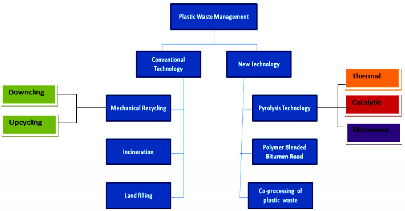
The world is today faced with the problem of plastic waste pollution more than ever before. Global plastic production continues to accelerate, despite the fact that recycling rates are comparatively low, with only about 15% of the 400 million tonnes of plastic currently produced annually being recycled. Although recycling rates have been steadily growing over the last 30 years, the rate of global plastic production far outweighs this, meaning that more and more plastic is ending up in dump sites, landfills and finally into the environment, where it damages the ecosystem. Better end-of-life options for plastic waste are needed to help support current recycling efforts and turn the tide on plastic waste. A promising emerging technology is plastic pyrolysis; a chemical process that breaks plastics down into their raw materials. Key products are liquid resembling crude oil, which can be burned as fuel and other feedstock which can be used for so many new chemical processes, enabling a closed-loop process. The experimental results on the pyrolysis of thermoplastic polymers are discussed in this review with emphasis on single and mixed waste plastics pyrolysis liquid fuel.
Citation: Wilson Uzochukwu Eze, Reginald Umunakwe, Henry Chinedu Obasi, Michael Ifeanyichukwu Ugbaja, Cosmas Chinedu Uche, Innocent Chimezie Madufor. Plastics waste management: A review of pyrolysis technology[J]. Clean Technologies and Recycling, 2021, 1(1): 50-69. doi: 10.3934/ctr.2021003
The world is today faced with the problem of plastic waste pollution more than ever before. Global plastic production continues to accelerate, despite the fact that recycling rates are comparatively low, with only about 15% of the 400 million tonnes of plastic currently produced annually being recycled. Although recycling rates have been steadily growing over the last 30 years, the rate of global plastic production far outweighs this, meaning that more and more plastic is ending up in dump sites, landfills and finally into the environment, where it damages the ecosystem. Better end-of-life options for plastic waste are needed to help support current recycling efforts and turn the tide on plastic waste. A promising emerging technology is plastic pyrolysis; a chemical process that breaks plastics down into their raw materials. Key products are liquid resembling crude oil, which can be burned as fuel and other feedstock which can be used for so many new chemical processes, enabling a closed-loop process. The experimental results on the pyrolysis of thermoplastic polymers are discussed in this review with emphasis on single and mixed waste plastics pyrolysis liquid fuel.

| [1] | Philippe C (2019) The history of plastics: from the capitol to the Tarpeian Rock. Field Actions Sci Rep 19: 6-11. |
| [2] |
Livingston E, Desai A, Berkwits M (2020) Sourcing personal protective equipment during the COVID-19 pandemic. JAMA 323: 1912-1914. doi: 10.1001/jama.2020.5317

|
| [3] |
Czigány T, Ronkay F (2020) The coronavirus and plastics. Express Polym Lett 14: 510-511. doi: 10.3144/expresspolymlett.2020.41
|
| [4] | Gaiya JD, Eze WU, Ekpenyong SA, et al. (2018) Effect of carbon particles on electrical conductivity of unsaturated polyester resin composite national engineering conference, 142-144. |
| [5] | Gaiya JD, Eze WU, Oyegoke T, et al. (2021) Assessment of the dielectric properties of polyester/metakaolin composite. Eur J Mater Sci Eng 6: 19-29. |
| [6] |
Babayemi JO, Nnorom IC, Osibanjo O, et al. (2019) Ensuring sustainability in plastics use in Africa: consumption, waste generation, and projections. Environ Sci Eur 31: 60. doi: 10.1186/s12302-019-0254-5
|
| [7] | Li WC, Tse HF, Fok L (2016) Plastic waste in the marine environment: a review of sources, occurrence and effects. Sci Total Environ 567: 333-349. |
| [8] |
Geyer R, Jambeck JR, Law KL (2017) Production, use, and fate of all plastics ever made. Sci Adv 3: 1-5. doi: 10.1126/sciadv.1700782
|
| [9] |
Miandad R, Barakat MA, Aburiazaiza AS, et al. (2016) Catalytic pyrolysis of plastic waste: a review. Process Safety Environ Protect 102: 822-838. doi: 10.1016/j.psep.2016.06.022
|
| [10] |
Ratnasari DK, Nahil MA, Williams PT (2016) Catalytic pyrolysis of waste plastics using staged catalysis for production of gasoline range hydrocarbon oils. J Anal Appl Pyrolysis 124: 631-637. doi: 10.1016/j.jaap.2016.12.027
|
| [11] |
Kawai K, Tasaki T (2016) Revisiting estimates of municipal solid waste generation per capita and their reliability. J Mater Cycles Waste Manage 18: 1-13. doi: 10.1007/s10163-015-0355-1
|
| [12] | ESI Africa (2018) S. Africa: 1.144 m tonnes of recyclable plastic dumped in landfills. Available from: https://www.esi-africa.com/top-stories/s-africa-1-144m-tonnes-of-recyclable-plastic-dumped-in-landfills/. |
| [13] |
Wagner M, Scherer C, Alvarez-Munoz D, et al (2014) Microplastics in freshwater ecosystems: what we know and what we need to know. Environ Sci Eur 26: 9. doi: 10.1186/2190-4715-26-9
|
| [14] |
Wrighta SL, Thompson RC, Galloway TS (2013) The physical impacts of microplastics on marine organisms: a review. Environ Pollut 178: 483-492. doi: 10.1016/j.envpol.2013.02.031
|
| [15] | Werner S, Budziak A, van Franeker J, et al. (2016) Harm caused by marine litter. MSFD GES TG marine litter—Thematic Report; JRC Technical report; EUR 28317 EN. |
| [16] |
Anderson JC, Park BJ, Palace VP (2016) Microplastics in aquatic environments: implications for Canadian ecosystems. Environ Pollut 218: 269-280. doi: 10.1016/j.envpol.2016.06.074
|
| [17] |
Srivastava V, Ismail SA, Singh P, et al. (2015) Urban solid waste management in the developing world with emphasis on India: Challenges and opportunities. Rev Environ Sci Bio-Technol 14: 317-337. doi: 10.1007/s11157-014-9352-4
|
| [18] |
Schuga TT, Janesickb A, Blumbergb B, et al. (2011) Endocrine disrupting chemicals and disease susceptibility. J Steroid Biochem Mol Biol 127: 204-215. doi: 10.1016/j.jsbmb.2011.08.007
|
| [19] | Willner SA, Blumberg B (2019) Encyclopedia of endocrine diseases (second edition). |
| [20] |
Verma R, Vinoda KS, Papireddy M, et al. (2016) Toxic pollutants from plastic waste-a review. Procedia Environ Sci 35: 701-708. doi: 10.1016/j.proenv.2016.07.069
|
| [21] | Conlon K (2021) A social systems approach to sustainable waste management: leverage points for plastic reduction in Colombo, Sri Lanka. Int J Sustainable Dev World Ecol 1-19. |
| [22] |
Clapp J, Swanston L (2009) Doing away with plastic shopping bags: international patterns of norm emergence and policy implementation. Environ Polit 18: 315-332. doi: 10.1080/09644010902823717
|
| [23] |
Imam A, Mohammed B, Wilson DC, et al. (2008) Solid waste management in Abuja, Nigeria. Waste Manage 28: 468-472. doi: 10.1016/j.wasman.2007.01.006
|
| [24] |
Chida M (2011) Sustainability in retail: The failed debate around plastic shopping bags. Fashion Pract 3: 175-196. doi: 10.2752/175693811X13080607764773
|
| [25] | Devy K, Nahil MA, Williams PT (2016) Catalytic pyrolysis of waste plastics using staged catalysis for production of gasoline range hydrocarbon oils. J Anal Appl Pyrolysis 124: 631-637. |
| [26] |
Eze WU, Madufor IC, Onyeagoro GN, et al. (2020) The effect of Kankara zeolite-Y-based catalyst on some physical properties of liquid fuel from mixed waste plastics (MWPs) pyrolysis. Polym Bull 77: 1399-1415. doi: 10.1007/s00289-019-02806-y
|
| [27] |
Eze WU, Madufor IC, Onyeagoro GN, et al. (2021) Study on the effect of Kankara zeolite-Y-based catalyst on the chemical properties of liquid fuel from mixed waste plastics (MWPs) pyrolysis. Polym Bull 78: 377. doi: 10.1007/s00289-020-03116-4
|
| [28] |
Vasile C, Brebu M, Karayildirim T, et al. (2006) Feedstock recycling from plastic and thermoset fractions of used computers (I): pyrolysis. J Mater Cycles Waste Manage 8: 99-108. doi: 10.1007/s10163-006-0151-z
|
| [29] |
Teuten EL, Saquin JM, Knappe DR, et al. (2009) Transport and release of chemicals from plastics to the environment and to wildlife. Philos Trans R Soc Lond B Biol Sci 364: 2027-2045. doi: 10.1098/rstb.2008.0284
|
| [30] |
Hopewell J, Dvorak R, Kosior E (2009) Plastics recycling: challenges and opportunities. Philos Trans R Soc B 364: 2115-2126. doi: 10.1098/rstb.2008.0311
|
| [31] |
Valavanidid A, Iliopoulos N, Gotsis G, et al. (2008) Persistent free radicals, heavy metals and PAHs generated in particulate soot emissions and residual ash from controlled combustion of common type of plastics. J Hazard Mater 156: 277-284. doi: 10.1016/j.jhazmat.2007.12.019
|
| [32] |
Qureshi MS, Oasmaa A, Pihkola H, et al (2020) Pyrolysis of plastic waste: Opportunities and challenges. J Anal Appl Pyrolysis 152: 104804. doi: 10.1016/j.jaap.2020.104804
|
| [33] |
López A, de Marco I, Caballero BM, et al. (2011) Influence of time and temperature on pyrolysis of plastic wastes in a semi-batch reactor. Chem Eng J 173: 62-71. doi: 10.1016/j.cej.2011.07.037
|
| [34] |
Scott DS, Czernik SR, Piskorz J, et al. (1990) Fast pyrolysis of plastic wastes. Energy Fuels 4: 407-411. doi: 10.1021/ef00022a013
|
| [35] |
Santaweesuk C, Janyalertadun A (2017) The production of fuel oil by conventional slow pyrolysis using plastic waste from a municipal landfill. Int J Environ Sci Dev 8: 168-173. doi: 10.18178/ijesd.2017.8.3.941
|
| [36] |
Kunwar B, Moser BR, Chandrasekaran SR, et al. (2016) Catalytic and thermal depolymerization of low value post-consumer high density polyethylene plastic. Energy 111: 884-892. doi: 10.1016/j.energy.2016.06.024
|
| [37] |
Shah J, Jan MR, Mabood F, et al. (2010) Catalytic pyrolysis of LDPE leads to valuable resource recovery and reduction of waste problems. Energy Convers Manage 51: 2791-2801. doi: 10.1016/j.enconman.2010.06.016
|
| [38] |
Bow Y, Rusdianasari, Pujiastuti LS (2019) Pyrolysis of polypropylene plastic waste into liquid fuel. IOP Conf Ser: Earth Environ Sci 347: 012128. doi: 10.1088/1755-1315/347/1/012128
|
| [39] |
Honus S, Kumagai S, Fedorko G, et al. (2018) Pyrolysis gases produced from individual and mixed PE, PP, PS, PVC, and PET—Part I: Production and physical properties. Fuel 221: 346-360. doi: 10.1016/j.fuel.2018.02.074
|
| [40] |
Miandad R, Rehan M, Barakat MA, et al. (2019) Catalytic pyrolysis of plastic waste: Moving Toward Pyrolysis Based Biorefineries. Front Energy Res 7: 27. doi: 10.3389/fenrg.2019.00027
|
| [41] |
Olufemi AS, Olagboye S (2017) Thermal conversion of waste plastics into fuel oil. Int J Petrochem Sci Eng 2: 252-257. doi: 10.15406/ipcse.2017.02.00064
|
| [42] | Kaminsky W (1992) Plastics, recycling, In: Ullmann's encyclopedia of industrial chemistry, 57 73, Wiley-VCH, 3-52730-385-5, Germany. |
| [43] | Meredith R (1998) Engineers' handbook of industrial microwave heating, The Institution of Electrical Engineers, 0-85296-916-3, United Kindom. |
| [44] |
Ludlow-Palafox C, Chase HA (2001) Microwave-induced pyrolysis of plastic wastes. Ind Eng Chem Res 40: 4749-4756. doi: 10.1021/ie010202j
|
| [45] |
Hussain Z, Khan KM, Hussain K (2010) Microwave-metal interaction pyrolysis of polystyrene. J Anal Appl Pyrolysis 89: 39-43. doi: 10.1016/j.jaap.2010.05.003
|
| [46] | Undri A, Rosi L, Frediani M, et al. (2011) Microwave pyrolysis of polymeric materials, Microwave Heating, Usha Chandra, IntechOpen, DOI: 10.5772/24008. Available from: https://www.intechopen.com/books/microwave-heating/microwave-pyrolysis-of-polymeric-materials. |
| [47] |
Panda AK, Singh RK (2011) Catalytic performances of kaoline and silica alumina in the thermal degradation of polypropylene. J Fuel Chem Technol 39: 198-202. doi: 10.1016/S1872-5813(11)60017-0
|
| [48] | George M, Yusof IY, Papayannakos N, et al. (2001) Catalytic cracking of polyethylene over clay catalysts. Comparison with an Ultrastable Y Zeolite. Ind Eng Chem Res 40: 2220-2225. |
| [49] |
Kumar KP, Srinivas S (2020) Catalytic Co-pyrolysis of Biomass and Plastics (Polypropylene and Polystyrene) Using Spent FCC Catalyst. Energy Fuels 34: 460-473. doi: 10.1021/acs.energyfuels.9b03135
|
| [50] |
Yoshio U, Nakamura J, Itoh T, et al. (1999) Conversion of polyethylene into gasoline-range fuels by two-stage catalytic degradation using Silica−Alumina and HZSM-5 Zeolite. Ind Eng Chem Res 38: 385-390. doi: 10.1021/ie980341+
|
| [51] |
Uddin MA, Koizumi K, Murata K, et al. (1997) Thermal and catalytic degradation of structurally different types of polyethylene into fuel oil. Polym Degrad Stab 56: 37-44. doi: 10.1016/S0141-3910(96)00191-7
|
| [52] |
Rasul JM, Shah J, Gulab H (2010) Catalytic degradation of waste high-density polyethylene into fuel products using BaCO3 as a catalyst. Fuel Process Technol 91: 1428-1437. doi: 10.1016/j.fuproc.2010.05.017
|
| [53] |
Rasul JM, Shah J, Gulab H (2010) Degradation of waste High-density polyethylene into fuel oil using basic catalyst. Fuel 89: 474-480. doi: 10.1016/j.fuel.2009.09.007
|
| [54] |
Hakeem IG, Aberuagba F, Musa U (2018) Catalytic pyrolysis of waste polypropylene using Ahoko kaolin from Nigeria. Appl Petrochem Res 8: 203-210. doi: 10.1007/s13203-018-0207-8
|
| [55] |
Xue Y, Johnston P, Bai X (2017) Effect of catalyst contact mode and gas atmosphere during catalytic pyrolysis of waste plastics. Energy Convers Manage 142: 441-451. doi: 10.1016/j.enconman.2017.03.071
|
| [56] |
Akpanudoh NS, Gobin K, Manos G (2005) Catalytic degradation of plastic waste to liquid fuel over commercial cracking catalysts: Effect of polymer to catalyst ratio/acidity content. J Mol Catal A: Chem 235: 67-73. doi: 10.1016/j.molcata.2005.03.009
|
| [57] |
Bridgewater AV (2012) Review of fast pyrolysis of biomass and product upgrading. Biomass Bioenergy 38: 68-94. doi: 10.1016/j.biombioe.2011.01.048
|
| [58] |
Miskolczi N, Angyal A, Bartha L, et al. (2009) Fuel by pyrolysis of waste plastics from agricultural and packaging sectors in a pilot scale reactor. Fuel Process Technol 90: 1032-1040. doi: 10.1016/j.fuproc.2009.04.019
|
| [59] |
Chen D, Yin L, Wang H, et al. (2014) Pyrolysis technologies for municipal solid waste: a review. Waste Manage 34: 2466-2486. doi: 10.1016/j.wasman.2014.08.004
|
| [60] |
Achilias DS, Roupakias C, Megalokonomos P, et al. (2007) Chemical recycling of plastic wastes made from polyethylene (LDPE and HDPE) and polypropylene (PP). J Hazard Mater 149: 536-542. doi: 10.1016/j.jhazmat.2007.06.076
|
| [61] |
Lee SY (2001) Catalytic degradation of polystyrene over natural clinoptilolite zeolite. Polym Degrad Stab 74: 297-305. doi: 10.1016/S0141-3910(01)00162-8
|
| [62] | Christine C, Thomas S, Varghese S (2013) Synthesis of petroleum-based fuel from waste plastics and performance analysis in a CI engine. J Energy 2013: 608797. |
| [63] | Khan MZH, Sultana M, Al-Mamun MR, et al. (2016) Pyrolytic waste plastic oil and its diesel Blend: fuel characterization. J Environ Public Health 2016: 7869080. |
| [64] |
Panda AK, Alotaibi A, Kozhevnikov IV, et al. (2020) Pyrolysis of plastics to liquid fuel using sulphated zirconium hydroxide catalyst. Waste Biomass Valor 11: 6337-6345. doi: 10.1007/s12649-019-00841-4
|
| [65] | Sophonrat N (2018) Pyrolysis of mixed plastics and paper to produce fuels and other chemicals. Doctoral Dissertation, KTH Royal Institute of Technology School of Industrial Engineering and Management Department of Materials Science and Engineering Unit of Processes, Sweden. |
| [66] |
Supramono D, Nabil M, Setiadi A, et al. (2018) Effect of feed composition of co-pyrolysis of corncobs-polypropylene plastic on mass interaction between biomass particles and plastics. IOP Conf Ser: Earth Environ Sci 105: 012049 doi: 10.1088/1755-1315/105/1/012049
|
| [67] | Baiden (2018) Pyrolysis of plastic waste from medical services facilities into potential fuel and/or fuel additives. Master's Theses, 3696. Available from: https://scholarworks.wmich.edu/masters_theses/3696. |
| [68] |
Hopewell J, Dvorak R, Kosior E (2009) Plastics recycling: challenges and opportunities. Philos Trans R Soc London B Biol Sci 364: 2115-2126. doi: 10.1098/rstb.2008.0311
|
| [69] |
Demirbas A (2004) Pyrolysis of municipal plastic wastes for recovery of gasoline range hydrocarbons. J Anal Appl Pyrol 72: 97-102. doi: 10.1016/j.jaap.2004.03.001
|
| [70] |
Donaj PJ, Kaminsky W, Buzeto F, et al. (2012) Pyrolysis of polyolefins for increasing the yield of monomers' recovery. Waste Manage 32: 840-846. doi: 10.1016/j.wasman.2011.10.009
|
| [71] | Pratama NN, Saptoadi H (2014) Characteristics of waste plastics pyrolytic oil and its applications as alternative fuel on four cylinder diesel engines. Int J Renewable Energy Dev 3: 13-20. |
| [72] |
Wathakit K, Sukjit E, Kaewbuddee C, et al. (2021) Characterization and impact of waste plastic oil in a variable compression ratio diesel engine. Energies 14: 2230. doi: 10.3390/en14082230
|
| [73] |
Abnisa F, Wan Daud WMA, Arami-Niya A, et al. (2014) Recovery of liquid fuel from the aqueous phase of pyrolysis oil using catalytic conversion. Energy Fuels 28: 3074-3085. doi: 10.1021/ef5003952
|
| [74] | Alam M, Song J, Acharya R, et al. (2004) Combustion and emissions performance of low sulfur, ultra low sulfur and biodiesel blends in a DI diesel engine. SAE Trans 113: 1986-1997. |


Figures(4) / Tables(5)
Wilson Uzochukwu Eze, Reginald Umunakwe, Henry Chinedu Obasi, Michael Ifeanyichukwu Ugbaja, Cosmas Chinedu Uche, Innocent Chimezie Madufor. Plastics waste management: A review of pyrolysis technology[J]. Clean Technologies and Recycling, 2021, 1(1): 50-69. doi: 10.3934/ctr.2021003


 DownLoad: