Biophysical insights into nanomaterial-induced DNA damage: mechanisms, challenges, and future directions

James C.L. Chow; James C.L. Chow

doi:10.3934/biophy.2024019

AIMS Biophysics

2024, Volume 11, Issue 3: 340-369. doi: 10.3934/biophy.2024019

Previous Article Next Article

Review

Biophysical insights into nanomaterial-induced DNA damage: mechanisms, challenges, and future directions

James C.L. Chow ^{1,2
,
,}

1.
Department of Radiation Oncology, University of Toronto, Toronto, Ontario, Canada
2.
Radiation Medicine Program, Princess Margaret Cancer Centre, University Health Network, Toronto, Ontario, Canada

Received: 19 July 2024 Revised: 23 August 2024 Accepted: 06 September 2024 Published: 11 September 2024

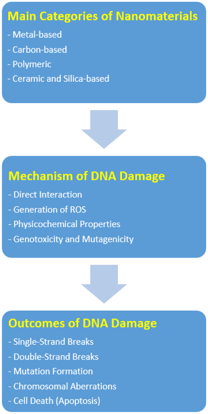
Nanomaterials have garnered significant attention due to their unique properties and wide-ranging applications in medicine and biophysics. However, their interactions with biological systems, particularly DNA, raise critical concerns about genotoxicity and potential long-term health risks. This review delves into the biophysical mechanisms underlying nanomaterial-induced DNA damage, highlighting recent insights, current challenges, and future research directions. We explore how the physicochemical properties of nanomaterials influence their interaction with DNA, the pathways through which they induce damage, and the biophysical methods employed to study these processes.

Keywords:

Citation: James C.L. Chow. Biophysical insights into nanomaterial-induced DNA damage: mechanisms, challenges, and future directions[J]. AIMS Biophysics, 2024, 11(3): 340-369. doi: 10.3934/biophy.2024019

Related Papers:

[1]	Erlin Guo, Cuixia Li, Patrick Ling, Fengqin Tang . Convergence rate for integrated self-weighted volatility by using intraday high-frequency data with noise. AIMS Mathematics, 2023, 8(12): 31070-31091. doi: 10.3934/math.20231590
[2]	Wenhui Feng, Xingfa Zhang, Yanshan Chen, Zefang Song . Linear regression estimation using intraday high frequency data. AIMS Mathematics, 2023, 8(6): 13123-13133. doi: 10.3934/math.2023662
[3]	Yue Li, Yunyan Wang . Strong consistency of the nonparametric kernel estimator of the transition density for the second-order diffusion process. AIMS Mathematics, 2024, 9(7): 19015-19030. doi: 10.3934/math.2024925
[4]	Oussama Bouanani, Salim Bouzebda . Limit theorems for local polynomial estimation of regression for functional dependent data. AIMS Mathematics, 2024, 9(9): 23651-23691. doi: 10.3934/math.20241150
[5]	Ahmed Ghezal, Mohamed balegh, Imane Zemmouri . Markov-switching threshold stochastic volatility models with regime changes. AIMS Mathematics, 2024, 9(2): 3895-3910. doi: 10.3934/math.2024192
[6]	Gaosheng Liu, Yang Bai . Statistical inference in functional semiparametric spatial autoregressive model. AIMS Mathematics, 2021, 6(10): 10890-10906. doi: 10.3934/math.2021633
[7]	Junke Kou, Hao Zhang . Wavelet estimations of the derivatives of variance function in heteroscedastic model. AIMS Mathematics, 2023, 8(6): 14340-14361. doi: 10.3934/math.2023734
[8]	Omar Alzeley, Ahmed Ghezal . On an asymmetric multivariate stochastic difference volatility: structure and estimation. AIMS Mathematics, 2024, 9(7): 18528-18552. doi: 10.3934/math.2024902
[9]	Jiajia Zhao, Zuoliang Xu . Calibration of time-dependent volatility for European options under the fractional Vasicek model. AIMS Mathematics, 2022, 7(6): 11053-11069. doi: 10.3934/math.2022617
[10]	Fatimah Alshahrani, Wahiba Bouabsa, Ibrahim M. Almanjahie, Mohammed Kadi Attouch . $k$ NN local linear estimation of the conditional density and mode for functional spatial high dimensional data. AIMS Mathematics, 2023, 8(7): 15844-15875. doi: 10.3934/math.2023809

Abstract

1. Introduction

Many complicated structures' memory and natural features may be realized using fractional calculus (FC), which studies integrals and derivatives of fractional orders ^[1,2]. Many recent FC applications have included analyzing the dynamics of large-scale physical events by converting derivatives and integrals from classical to non-integer order. Many branches of engineering and the physical sciences use it, including electric circuits, mathematical biology, control theory, robotics, viscoelasticity, flow models, relaxation, and signal processing ^[3,4]. Numerous mysterious ideas have been refined via the study of fractional calculus, for example, logistic regression, Malthusian growth, and blood alcohol concentration, all of which have shown that fractional operators outperform integer-order operators ^[5,6].

Derivatives of fractional order such as Riemann-Liouville, Atangana Baleanu, Caputo, Hilfer, Grunwald-Letnikov, Caputo Fabrizio, and Riemann-Liouville are among the numerous that have recently been proposed ^[7,8]. Since all fractional derivatives may be reduced in Caputo's meaning with minor parametric adjustments, the fractional derivative of Caputo is the essential principle of FC to investigate fractional differential equations (FDEs). Caputo's operator, which has numerous applications to model various physical models, possesses a power-law kernel. To address this difficulty, the alternative fractional differential operator ^[9] was developed, which consists of a Mittag-Leffler kernel and an exponentially decaying kernel. Caputo-Fabrizio (CF) and Atangana-Baleanu are operators characterized by their non-singular kernels. These operators have been widely applied in analyzing diverse problem classes, including but not limited to biology, economics, geophysics, and bioengineering ^[10].

Korteweg and de Vries introduced the KdV equation in 1895 to formulate a model for Russell's soliton phenomenon, encompassing water waves of long and small amplitude. Solitons are classified as stable solitary waves, signifying their particle-like nature ^[11]. Various applied disciplines, including plasma physics, fluid dynamics, quantum mechanics, and optics, implement the KdV equations ^[12]. Particle physics has employed the fifth-order KdV equations to analyze many nonlinear phenomena ^[13]. Its function in the propagation of waves is crucial ^[14]. The authors find third-order and fifth-order dispersive terms in the KdV form equation pertinent to the magneto-acoustic wave problem. Furthermore, these dispersive terms manifest themselves in the vicinity of critical angle propagation ^[15]. An electrically conducting fluid, plasma is also dynamic and quasi-neutral. Ions, electrons, and neutral particles comprise it. Due to the electrical conductivity exhibited by plasma, it includes both electric and magnetic regions. The variety of particles and regions supports diverse types of plasma waves. A magnetic lock is a less longitudinal ion dispersion. In the low magnetic field range, the magneto-acoustic wave exhibits characteristics of an ion acoustic wave ^[16,17]. However, at low temperatures, it transforms into an Alfven wave.

Equivalent to the general model for the investigation of magnetic characteristics of acoustic waves with surface tension is the fifth order of KdV. According to a recent investigation ^[18,19], the solutions to the equation above concerning traveling waves persist beyond infinity. The following are two widely recognized types of fifth-order KdV equations ^[20,21]:

$\begin{equation} \begin{split} &D_{{\Omega}}^{p} \eta({\epsilon}, {\Omega})-\frac{\partial ^5\eta({\epsilon}, {\Omega})}{\partial \epsilon^5}+\eta({\epsilon}, {\Omega}) \frac{\partial ^3\eta({\epsilon}, {\Omega})}{\partial \epsilon^3}+\eta({\epsilon}, {\Omega}) \frac{\partial \eta({\epsilon}, {\Omega})}{\partial \epsilon} = 0, \ \ 0 < p \leq 1. \end{split} \end{equation}$

(1.1)

$\begin{equation} \begin{split} &D_{{\Omega}}^{p} \eta({\epsilon}, {\Omega})+\frac{\partial ^5\eta({\epsilon}, {\Omega})}{\partial \epsilon^5}-\eta({\epsilon}, {\Omega}) \frac{\partial ^3\eta({\epsilon}, {\Omega})}{\partial \epsilon^3}+\eta({\epsilon}, {\Omega}) \frac{\partial \eta({\epsilon}, {\Omega})}{\partial \epsilon} = 0, \ \ 0 < p \leq 1. \end{split} \end{equation}$

(1.2)

Here, Eqs (1.1) and (1.2) are called the Kawahara and KdV equation of fifth-order, respectively. The extreme nonlinearity of these mathematical models makes it difficult to find suitable analytical methods. Researchers have developed and implemented several techniques for solving nonlinear and linear equations of KdV in the past ten years. These techniques include the variational iteration method ^[21], the multi-symplectic method ^[22], He's homotopy perturbation method ^[23], and the Exp-function method ^[24].

Omar Abu Arqub established residual power series method (RPSM) in 2013 ^[25]. It is created by merging the residual error function with the Taylor series. According to ^[26], an infinite convergence series solves differential equations (DEs). The development of novel RPSM algorithms has been prompted by several DEs, including KdV Burger's equation, fuzzy DEs, Boussinesq DEs, and numerous others ^[27,28]. The goal of these algorithms is to provide efficient and accurate estimates.

A novel strategy for solving FDEs was established by integrating two effective methods. Some approaches that fall into these categories include those that use the natural transform ^[29], the Laplace transform with RPSM ^[30], and the homotopy perturbation method ^[31]. In this work, we used a novel combination method known as the Abdooh residual power series method (ARPSM) to discover approximation and precise solutions for time-fractional nonlinear partial differential equations (PDEs). This innovative method is significant because it combines the Aboodh transform technique with the RPSM ^[32,33].

The computing effort and complexity needed are significant issues with the previously mentioned approaches. Our suggested Aboodh transform iterative method (ATIM) ^[34] is this work's unique aspect that solves the Kawahara and KdV equations of fractional order. By integrating the Aboodh transform with the new iterative technique, this strategy significantly reduces the computing effort and complexity required. According to ^[35,36], the suggested approach yields a convergent series solution.

The ARPSM and the ATIM are the two most straightforward approaches to solving fractional DEs. These methods fully and immediately explain the symbolic terms used in analytical solutions and offer numerical solutions to PDEs. This paper assesses ATIM and ARPSM's efficacy in solving the fifth-order KdV and Kawahara equations.

The fifth-order KdV and Kawahara equations are solved using ARPSM and ATIM. These methods provide more precise numerical answers when compared with other numerical techniques. Additionally, a comparison analysis is performed on the numerical findings. The suggested approaches' findings are consistent with one another, which is a strong indicator of their efficacy and reliability. For various values of fractional-order derivatives, there is additional graphical importance. Therefore, the methods are accurate, easy to implement, not affected by computational error phases, and quick. This study lays the groundwork for researchers to quickly solve various PDEs.

2. Basics of fractional calculus

Definition 2.1. ^[37] Assume that $\eta({{\epsilon}}, {{\Omega}})$ is an exponential order continuous function. The definition of the Aboodh transform (AT), assuming $\sigma\geq0$ for $\eta({{\epsilon}}, {{\Omega}})$ , is as follows:

$A[\eta({{\epsilon}}, {{\Omega}})] = \Psi({{\epsilon}},\xi) = \frac{1}{\xi}\displaystyle{\int}_{0}^{\infty}\eta({{\epsilon}}, {{\Omega}})e^{-{{\Omega}}\xi}d{{\Omega}},\ \ {r}_{1}\leq\xi\leq{r}_{2}.$

The Aboodh inverse transform (AIT) is given as:

$A^{-1}[\Psi({{\epsilon}},\xi)] = \eta({{\epsilon}}, {{\Omega}}) = \frac{1}{2\pi i}\displaystyle{\int}_{u-i\infty}^{u+i\infty}\Psi({{\epsilon}}, {{\Omega}})\xi e^{{{\Omega}}\xi}d{{\Omega}},$

where ${{\epsilon}} = ({{\epsilon}}_{1}, {{\epsilon}}_{2}, \cdots, {{\epsilon}}_{p})\in \mathbb{R}^{p}$ and $p\in\mathbb{N}$ .

Lemma 2.1. ^[38,39] It is assumed that there exist two exponentially ordered, piecewise continuous functions $\eta_{1}({{\epsilon}}, \Omega)$ and $\eta_{2}({{\epsilon, \Omega}})$ on $[0, \infty]$ . Let $A[\eta_{1}({{\epsilon}}, {{\Omega}})] = \Psi_{1}({{\epsilon}}, {{\Omega}}), A[\eta_{2}({{\epsilon}}, {{\Omega}})] = \Psi_{2}({{\epsilon}}, {{\Omega}})$ , and $\chi_{1}, \chi_{2}$ be arbitrary constants. These characteristics are thus true:

(1) $A[\chi_{1}\eta_{1}({{\epsilon}}, {{\Omega}})+\chi_{2}\eta_{2}({{\epsilon}}, {{\Omega}})] = \chi_{1}\Psi_{1}({{\epsilon}}, \xi)+\chi_{2}\Psi_{2}({{\epsilon}}, {{\Omega}})$ ,

(2) $A^{-1}[\chi_{1}\Psi_{1}({{\epsilon}}, {{\Omega}})+\chi_{2}\Psi_{2}({{\epsilon}}, {{\Omega}})] = \chi_{1}\eta_{1}({{\epsilon}}, \xi)+\chi_{2}\eta_{2}({{\epsilon}}, {{\Omega}})$ ,

(3) $A[J_{{{\Omega}}}^{{p}}\eta({{\epsilon}}, {{\Omega}})] = \frac{\Psi({{\epsilon}}, \xi)}{\xi^{{p}}}$ ,

(4) $A[D_{{{\Omega}}}^{{p}}\eta({{\epsilon}}, {{\Omega}})] = \xi^{{p}}\Psi({{\epsilon}}, \xi)-\sum_{K = 0}^{r-1}\frac{\eta^{K}({{\epsilon}}, 0)}{\xi^{K-{p}+2}}, r-1 < {p}\leq r, \ r\in \mathbb{N}$ .

Definition 2.2. ^[40] In terms of order $p$ , the function $\eta({{\epsilon}}, {{\Omega}})$ has derivative of fractional order as stated by Caputo.

$D_{{{\Omega}}}^{{p}}\eta({{\epsilon}}, {{\Omega}}) = J_{{{\Omega}}}^{m-{p}}\eta^{(m)}({{\epsilon}}, {{\Omega}}), \ m-1 < {p}\leq m,\ r\geq 0,$

where ${{\epsilon}} = ({{\epsilon}}_{1}, {{\epsilon}}_{2}, \cdots, {{\epsilon}}_{p})\in \mathbb{R}^{p}$ and $p, m\in R, J_{{{\Omega}}}^{m-{p}}$ is the integral of the Riemann-Liouville of $\eta({{\epsilon}}, {{\Omega}})$ .

Definition 2.3. ^[41] The representation of power series is composed of the following structure.

$\sum\limits_{r = 0}^{\infty}\hbar_{r}({{\epsilon}})({{\Omega}}-{{\Omega}}_{0})^{r{p}} = 1+\hbar_{1}({{\Omega}}-{{\Omega}}_{0})^{{p}}+\hbar_{2}({{\Omega}}-{{\Omega}}_{0})^{2{p}} +\cdots,$

where ${{\epsilon}} = ({{\epsilon}}_{1}, {{\epsilon}}_{2}, \cdots, {{\epsilon}}_{p})\in \mathbb{R}^{p}$ and $p\in \mathbb{N}$ . This is known as the multiple fractional power series concerning ${{\Omega}}_{0}$ , where ${{\Omega}}$ and $\hbar_{r}({{\epsilon}})'s$ are variable and series coefficients, respectively.

Lemma 2.2. Consider the exponential order function is denoted as $\eta({{\epsilon}}, {{\Omega}})$ . $A[\eta({{\epsilon}}, {{\Omega}})] = \Psi({{\epsilon}}, \xi)$ is the description of the AT in this case. Hence,

$\begin{equation} A[D_{{{\Omega}}}^{r{p}}\eta({{\epsilon}}, {{\Omega}})] = \xi^{r{p}}\Psi({{\epsilon}},\xi)-\sum\limits_{j = 0}^{r-1}\xi^{{p}(r-j)-2}D_{{{\Omega}}}^{j{p}}\eta({{\epsilon}},0), 0 < {p}\leq 1, \end{equation}$

(2.1)

where ${{\epsilon}} = ({{\epsilon}}_{1}, {{\epsilon}}_{2}, \cdots, {{\epsilon}}_{p})\in \mathbb{R}^{p}$ and $p\in \mathbb{N}$ and $D_{{{\Omega}}}^{r{p}} = D_{{{\Omega}}}^{{p}}.D_{{{\Omega}}}^{{p}}.\cdots.D_{{{\Omega}}}^{{p}}(r-times)$

Proof. By using the induction method, we have to prove Eq (2.1). In Eq (2.1), substitute $r = 1$ .

$A[D_{{{\Omega}}}^{{p}}\eta({{\epsilon}}, {{\Omega}})] = \xi^{{p}}\Psi({{\epsilon}},\xi)-\xi^{{p}-2}\eta({{\epsilon}},0)-\xi^{{p}-2}D_{{{\Omega}}}^{{p}}\eta({{\epsilon}},0).$

On the bases of Lemma 2.1, Eq (2.1) for $r = 1$ holds true. Put $r = 2$ in Eq (2.1).

$\begin{equation} A[D_{r}^{2{p}}\eta({{\epsilon}}, {{\Omega}})] = \xi^{2{p}}\Psi({{\epsilon}},\xi)-\xi^{2{p}-2}\eta({{\epsilon}},0)-\xi^{{p}-2}D_{{{\Omega}}}^{{p}}\eta({{\epsilon}},0). \end{equation}$

(2.2)

From left-hand side (LHS) of Eq (2.2), we obtain:

$\begin{equation} LHS = A[D_{{{\Omega}}}^{2{p}}\eta({{\epsilon}}, {{\Omega}})]. \end{equation}$

(2.3)

The expressions for Eq (2.3) are as follows:

$\begin{equation} LHS = A[D_{{{\Omega}}}^{{p}}\eta({{\epsilon}}, {{\Omega}})]. \end{equation}$

(2.4)

Assume

$\begin{equation} z({{\epsilon}}, {{\Omega}}) = D_{{{\Omega}}}^{{p}}\eta({{\epsilon}}, {{\Omega}}). \end{equation}$

(2.5)

This makes Eq (2.4) as

$\begin{equation} LHS = A[D_{{{\Omega}}}^{{p}}z({{\epsilon}}, {{\Omega}})]. \end{equation}$

(2.6)

From the definition of the derivative of Caputo, we make changes in Eq (2.6).

$\begin{equation} LHS = A[J^{1-{p}}z^{'}({{\epsilon}}, {{\Omega}})]. \end{equation}$

(2.7)

By applying the Riemann-Liouville integral Eq (2.7), we obtain:

$\begin{equation} LHS = \frac{A[z^{'}({{\epsilon}}, {{\Omega}})]}{\xi^{1-{p}}}. \end{equation}$

(2.8)

By using the AT feature of differentiability, Eq (2.8) is modified:

$\begin{equation} {{LHS = \xi^{{p}}Z({{\epsilon}},\xi)-\frac{z({{\epsilon}},0)}{\xi^{2-{p}}}.}} \end{equation}$

(2.9)

From Eq (2.5), we derive:

$Z({{\epsilon}},\xi) = \xi^{{p}}\Psi({{\epsilon}},\xi)-\frac{\eta({{\epsilon}},0)}{\xi^{2-{p}}},$

where $A[z({{\epsilon}}, {{\Omega}})] = Z({{\epsilon}}, \xi)$ . Hence, Eq (2.9) becomes

$\begin{equation} LHS = \xi^{2{p}}\Psi({{\epsilon}},\xi)-\frac{\eta({{\epsilon}},0)}{\xi^{2-2{p}}}-\frac{D_{{{\Omega}}}^{{p}}\eta({{\epsilon}},0)}{\xi^{2-{p}}}. \end{equation}$

(2.10)

Let's suppose Eq (2.1) holds true for $r = K$ . Substitute $r = K$ in Eq (2.1):

$\begin{equation} A[D_{{{\Omega}}}^{K{p}}\eta({{\epsilon}}, {{\Omega}})] = \xi^{K{p}}\Psi({{\epsilon}},\xi)-\sum\limits_{j = 0}^{K-1}\xi^{{p}(K-j)-2}D_{{{\Omega}}}^{j{p}}D_{{{\Omega}}}^{j{p}}\eta({{\epsilon}},0),\ 0 < {p}\leq1. \end{equation}$

(2.11)

Substituting $r = K+1$ in Eq (2.1):

$\begin{equation} A[D_{{{\Omega}}}^{(K+1){p}}\eta({{\epsilon}}, {{\Omega}})] = \xi^{(K+1){p}}\Psi({{\epsilon}},\xi)-\sum\limits_{j = 0}^{K}\xi^{{p}((K+1)-j)-2}D_{{{\Omega}}}^{j{p}}\eta({{\epsilon}},0). \end{equation}$

(2.12)

After analyzing Eq (2.12)'s LHS, we deduce

$\begin{equation} LHS = A[D_{{{\Omega}}}^{K{p}}(D_{{{\Omega}}}^{K{p}})]. \end{equation}$

(2.13)

Let

$D_{{{\Omega}}}^{K{p}} = g({{\epsilon}}, {{\Omega}}).$

By Eq (2.13), we drive

$\begin{equation} LHS = A[D_{{{\Omega}}}^{{p}}g({{\epsilon}}, {{\Omega}})]. \end{equation}$

(2.14)

By using the integral of the Riemann-Liouville and derivative of Caputo on Eq (2.14), the subsequent result can be obtained.

$\begin{equation} LHS = \xi^{{p}}A[D_{{{\Omega}}}^{K{p}}\eta({{\epsilon}}, {{\Omega}})]-\frac{g({{\epsilon}},0)}{\xi^{2-{p}}}. \end{equation}$

(2.15)

To get Eq (2.15), use Eq (2.11).

$\begin{equation} LHS = \xi^{r{p}}\Psi({{\epsilon}},\xi)-\sum\limits_{j = 0}^{r-1}\xi^{{p}(r-j)-2}D_{{{\Omega}}}^{j{p}}\eta({{\epsilon}},0). \end{equation}$

(2.16)

In addition, Eq (2.16) produces the subsequent outcome.

$LHS = A[D_{{{\Omega}}}^{r{p}}\eta({{\epsilon}},0)].$

Thus, for $r = K+1$ , Eq (2.1) holds. For all positive integers, Eq (2.1) holds true according to the mathematical induction technique. □

A deeper understanding of the ARPSM and multiple fractional Taylor series (MFTS) are given as follow.

Lemma 2.3. Consider the function $\eta({{\epsilon}}, {{\Omega}})$ is an exponential order. $A[\eta({{\epsilon}}, {{\Omega}})] = \Psi({{\epsilon}}, \xi)$ is the expression that signifies the AT of $\eta({{\epsilon}}, {{\Omega}})$ . AT is represented as follows in MFTS notation:

$\begin{equation} \Psi({{\epsilon}},\xi) = \sum\limits_{r = 0}^{\infty}\frac{\hbar_{r}({{\epsilon}})}{\xi^{r{p}+2}}, \xi > 0, \end{equation}$

(2.17)

where, ${{\epsilon}} = (s_{1}, {{\epsilon}}_{2}, \cdots, {{\epsilon}}_{p})\in\mathbb{R}^{p}, \ p\in \mathbb{N}$ .

Proof. Consider the Taylor's series:

$\begin{equation} \eta({{\epsilon}}, {{\Omega}}) = \hbar_{0}({{\epsilon}})+\hbar_{1}({{\epsilon}})\frac{{{\Omega}}^{{p}}}{\Gamma[{p}+1]}AA+\hbar_{2}({{\epsilon}})\frac{{{\Omega}}^{2{p}}}{\Gamma[2{p}+1]}+\cdots. \end{equation}$

(2.18)

The subsequent equality is produced when the AT is applied to Eq (2.18):

$A\left[\eta({{\epsilon}}, {{\Omega}})\right] = A\left[\hbar_{0}({{\epsilon}})\right]+A\left[\hbar_{1}({{\epsilon}})\frac{{{\Omega}}^{{p}}}{\Gamma[{p}+1]}\right]+A\left[\hbar_{1}({{\epsilon}}) \frac{{{\Omega}}^{2{p}}}{\Gamma[2{p}+1]}\right]+\cdots.$

This is achieved by utilizing the AT's features.

$A\left[\eta({{\epsilon}}, {{\Omega}})\right] = \hbar_{0}({{\epsilon}})\frac{1}{\xi^{2}}+\hbar_{1}({{\epsilon}})\frac{1}{\Gamma[{p}+1]}\frac{1}{\xi^{{p}+2}}+\hbar_{2}({{\epsilon}}) \frac{1}{\Gamma[2{p}+1]}\frac{1}{\xi^{2{p}+2}}\cdots.$

Hence, by Eq (2.17), a new Taylor's series is obtained: □

Lemma 2.4. Let the multiple fractional power series (MFPS) be expressed in terms of Taylor's series new form Eq (2.17), $A[\eta(\epsilon, \Omega)] = \Psi(\epsilon, \xi)$ .

$\begin{equation} \hbar_{0}({{\epsilon}}) = \lim\limits_{\xi\rightarrow \infty}\xi^2\Psi({{\epsilon}},\xi) = \eta({{\epsilon}},0). \end{equation}$

(2.19)

Proof. Let's suppose the Taylor's series:

$\begin{equation} \hbar_{0}({{\epsilon}}) = \xi^2\Psi({{\epsilon}},\xi)-\frac{\hbar_{1}({{\epsilon}})}{\xi^{{p}}}-\frac{\hbar_{2}({{\epsilon}})}{\xi^{2{p}}}-\cdots. \end{equation}$

(2.20)

As denoted by Eq (2.20), the necessary solution can be obtained by employing $lim_{x\rightarrow \infty}$ in Eq (2.19) and performing a short calculation. □

Theorem 2.5. The following is an MFPS representation of the function $A[\eta({{\epsilon}}, {{\Omega}})] = \Psi({{\epsilon}}, \xi)$ :

$\Psi({{\epsilon}},\xi) = \sum\limits_{0}^{\infty}\frac{\hbar_{r}({{\epsilon}})}{\xi^{r{p}+2}}, \ \xi > 0,$

where ${{\epsilon}} = ({{\epsilon}}_{1}, {{\epsilon}}_{2}, \cdots, {{\epsilon}}_{p})\in\mathbb{R}^p$ and $p\in\mathbb{N}$ . Then, we have

$\hbar_{r}({{\epsilon}}) = D_{r}^{r{p}}\eta({{\epsilon}},0),$

where, $D_{{{\Omega}}}^{r{p}} = D_{{{\Omega}}}^{{p}}.D_{{{\Omega}}}^{{p}}.\cdots.D_{{{\Omega}}}^{{p}}(r-times)$ .

Proof. Let's suppose the Taylor's series:

$\begin{equation} \hbar_{1}({{\epsilon}}) = \xi^{{p}+2}\Psi({{\epsilon}},\xi)-\xi^{{p}}\hbar_{0}({{\epsilon}})-\frac{\hbar_{2}({{\epsilon}})}{\xi^{{p}}}-\frac{\hbar_{3}({{\epsilon}})}{\xi^{2{p}}}- \cdots \end{equation}$

(2.21)

$\lim_{\xi\rightarrow \infty}$ , is applied to Eq (2.21), and we get

$\hbar_{1}({{\epsilon}}) = \lim\limits_{\xi\rightarrow \infty}(\xi^{{p}+2}\Psi({{\epsilon}},\xi)-\xi^{{p}}\hbar_{0}({{\epsilon}}))-\lim\limits_{\xi\rightarrow \infty}\frac{\hbar_{2}({{\epsilon}})}{\xi^{{p}}} -\lim\limits_{\xi\rightarrow \infty}\frac{\hbar_{3}({{\epsilon}})}{\xi^{2{p}}}- \cdots.$

The equality that results from taking the limit is as follows:

$\begin{equation} \hbar_{1}({{\epsilon}}) = \lim\limits_{\xi\rightarrow \infty}(\xi^{{p}+2}\Psi({{\epsilon}},\xi)-\xi^{{p}}\hbar_{0}({{\epsilon}})). \end{equation}$

(2.22)

Using Lemma 2.2, we obtain:

$\begin{equation} \hbar_{1}({{\epsilon}}) = \lim\limits_{\xi\rightarrow \infty}(\xi^2A[D_{{{\Omega}}}^{{p}}\eta({{\epsilon}}, {{\Omega}})](\xi)). \end{equation}$

(2.23)

Furthermore, the Eq (2.23) is modified using Lemma 2.3.

$\hbar_{1}({{\epsilon}}) = D_{{{\Omega}}}^{{p}}\eta({{\epsilon}},0).$

Using Taylor's series and applying $limit_{\xi\rightarrow \infty}$ again, we obtain:

$\hbar_{2}({{\epsilon}}) = \xi^{2{p}+2}\Psi({{\epsilon}},\xi)-\xi^{2{p}}\hbar_{0}({{\epsilon}})-\xi^{{p}}\hbar_{1}({{\epsilon}})-\frac{\hbar_{3}({{\epsilon}})}{\xi^{{p}}}- \cdots.$

Lemma 2.3 gives us the result

$\begin{equation} \hbar_2({{\epsilon}}) = \lim\limits_{\xi\rightarrow \infty}\xi^2(\xi^{2{p}}\Psi({{\epsilon}},\xi)-\xi^{2{p}-2}\hbar_{0}({{\epsilon}})-\xi^{{p}-2}\hbar_{1}({{\epsilon}})). \end{equation}$

(2.24)

Equation (2.24) is transformed using Lemmas 2.2 and Eq (2.4).

$\hbar_{2}({{\epsilon}}) = D_{{{\Omega}}}^{2{p}}\eta({{\epsilon}},0).$

Apply the same procedure and Taylor series, and we obtain:

$\hbar_{3}({{\epsilon}}) = \lim\limits_{\xi\rightarrow \infty}\xi^2(A[D_{{{\Omega}}}^{2{p}}\eta({{\epsilon}},{p})](\xi)).$

Finally, we get:

$\hbar_{3}({{\epsilon}}) = D_{{{\Omega}}}^{3{p}}\eta({{\epsilon}},0).$

In general,

$\hbar_{r}({{\epsilon}}) = D_{{{\Omega}}}^{r{p}}\eta({{\epsilon}},0),$

is proved. □ The new Taylor series has the conditions for the convergence given in the subsequent theorem.

Theorem 2.6. The expression for MFTS is given in Lemma 2.3 and can be expressed as: $A [\eta({{\epsilon}}, {{\Omega}})] = \Psi({{\epsilon}}, \xi)$ . When $|\xi^{a}A[D_{{{\Omega}}}^{(K+1){p}}\eta({{\epsilon}}, {{\Omega}})]|\leq T$ , $\forall$ $0 < {p} \leq 1$ , and $0 < \xi \leq s$ , $R_K({{\epsilon}}, \xi)$ is the residual of the new MFTS satisfying:

$|R_{K}({{\epsilon}},\xi)|\leq \frac{T}{\xi^{(K = 1){p}+2}}, \ 0 < \xi\leq s.$

Proof. For $r = 0, 1, 2, \cdots, K + 1$ , and $0 < \xi \leq s$ , we consider to define $A[D_{{{\Omega}}}^{r{p}}\eta({{\epsilon}}, {{\Omega}})](\xi)$ . Utilize the Taylor series to derive the subsequent relation:

$\begin{equation} R_K({{\epsilon}},\xi) = \Psi({{\epsilon}},\xi)-\sum\limits_{r = 0}^K\frac{\hbar_r({{\epsilon}})}{\xi^{r{p}+2}}. \end{equation}$

(2.25)

Apply Theorem 2.5 on Eq (2.25) to obtain:

$\begin{equation} R_K({{\epsilon}},\xi) = \Psi({{\epsilon}},\xi)-\sum\limits_{r = 0}^{K}\frac{D_{{{\Omega}}}^{r{p}}\eta({{\epsilon}},0)}{\xi^{r{p}+2}}. \end{equation}$

(2.26)

$\xi^{(K+1)a+2}$ is to be multiplied with Eq (2.26) to obtain the following form.

$\begin{equation} \xi^{{p}(K+1)+2}R_K({{\epsilon}},\xi) = \xi^{2}(\xi^{{p}(K+1)}\Psi({{\epsilon}},\xi)-\sum\limits_{r = 0}^{K}\xi^{{p}(K+1-r)-2}D_{{{\Omega}}}^{r{p}}\eta({{\epsilon}},0)). \end{equation}$

(2.27)

Equation (2.27) is modified with Lemma 2.2:

$\begin{equation} \xi^{{p}(K+1)+2}R_K({{\epsilon}},\xi) = \xi^{2}A[D_{{{\Omega}}}^{{p}(K+1)}\eta({{\epsilon}}, {{\Omega}})]. \end{equation}$

(2.28)

The absolute of Eq (2.28) gives us

$\begin{equation} |\xi^{{p}(K+1)+2}R_K({{\epsilon}},\xi)| = |\xi^{2}A[D_{{{\Omega}}}^{{p}(K+1)}\eta({{\epsilon}}, {{\Omega}})]|. \end{equation}$

(2.29)

By applying the conditions listed in Eq (2.29), the subsequent result is achieved.

$\begin{equation} \frac{-T}{\xi^{{p}(K+1)+2}}\leq R_K({{\epsilon}},\xi)\leq \frac{T}{\xi^{{p}(K+1)+2}}. \end{equation}$

(2.30)

Equation (2.30) yields the desired outcome.

$|R_K({{\epsilon}},\xi)|\leq \frac{T}{\xi^{{p}(K+1)+2}}.$

Therefore, new conditions for the series to converge are developed. □

3. Methodologies

3.1. ARPSM technique

In this paper, we explain how ARPSM rules formed the basis of our solution.

Step 1: Assume the general PDE:

$\begin{equation} D_{{{\Omega}}}^{q{p}}\eta({{\epsilon}}, {{\Omega}})+\vartheta({{\epsilon}})N(\eta)-\delta({{\epsilon}},\eta) = 0. \\ \end{equation}$

(3.1)

Step 2: Apply the AT on Eq (3.1):

$\begin{equation} A[D_{{{\Omega}}}^{q{p}}\eta({{\epsilon}}, {{\Omega}})+\vartheta({{\epsilon}})N(\eta)-\delta({{\epsilon}},\eta)] = 0. \\ \end{equation}$

(3.2)

Utilizing Lemma 2.1 to modify Eq (3.2),

$\begin{equation} \Psi({{\epsilon}},{s}) = \sum\limits_{j = 0}^{q-1}\frac{D_{{{\Omega}}}^{j}\eta({{\epsilon}},0)}{{s}^{q{p}+2}}-\frac{\vartheta({{\epsilon}})Y({s})}{{s}^{q{p}}}+\frac{F({{\epsilon}},{s})}{{s}^{q{p}}}, \end{equation}$

(3.3)

where $A[\delta({{\epsilon}}, \eta)] = F({{\epsilon}}, {s}), A[N(\eta)] = Y({s})$ .

Step 3: Equation (3.3) takes the following form:

$\Psi({{\epsilon}}, {s}) = \sum\limits_{r = 0}^{\infty}\frac{\hbar_r({{\epsilon}})}{{s}^{r{p}+2}}, \ {s} > 0. \\$

Step 4: Take the steps listed below:

$\hbar_0({{\epsilon}}) = \lim\limits_{{s}\rightarrow \infty}{s}^2 \Psi({{\epsilon}}, {s}) = \eta({{\epsilon}}, 0). \\$

Use Theorem 2.6 to obtain this form.

$\begin{array}{*{20}{c}} {\hbar_{1}({{\epsilon}}) = D_{{{\Omega}}}^{{p}}\eta({{\epsilon}}, 0),}\\ {\hbar_{2}({{\epsilon}}) = D_{{{\Omega}}}^{2{p}}\eta({{\epsilon}}, 0),}\\ {\vdots}\\ {\hbar_{w}({{\epsilon}}) = D_{{{\Omega}}}^{w{p}}\eta({{\epsilon}}, 0).} \end{array}$

Step 5: The $K^{th}$ truncated series $\Psi({{\epsilon}}, {s})$ can be obtained using the following expression:

$\Psi_{K}({{\epsilon}}, {s}) = \sum\limits_{r = 0}^{K}\frac{\hbar_r({{\epsilon}})}{{s}^{r{p}+2}}, \ {s} > 0,$

$\Psi_{K}({{\epsilon}}, {s}) = \frac{\hbar_{0}({{\epsilon}})}{{s}^{2}}+\frac{\hbar_{1}({{\epsilon}})}{{s}^{{p}+2}}+\cdots+\frac{\hbar_{w}({{\epsilon}})}{{s}^{w{p}+2}}+\sum\limits_{r = w+1}^{K} \frac{\hbar_r({{\epsilon}})}{{s}^{r{p}+2}}.$

Step 6: Note that the residual Aboodh function (RAF) (3.3) and the $K^{th}$ -truncated RAF must be considered independently to obtain:

$ARes({{\epsilon}}, {s}) = \Psi({{\epsilon}},{s})-\sum\limits_{j = 0}^{q-1}\frac{D_{{{\Omega}}}^{j}\eta({{\epsilon}},0)}{{s}^{j{p}+2}}+\frac{\vartheta({{\epsilon}})Y({s})}{{s}^{j{p}}}-\frac{F({{\epsilon}},{s})}{{s}^{j{p}}},$

and

$\begin{equation} ARes_{K}({{\epsilon}}, {s}) = \Psi_{K}({{\epsilon}},{s})-\sum\limits_{j = 0}^{q-1}\frac{D_{{{\Omega}}}^{j}\eta({{\epsilon}},0)}{{s}^{j{p}+2}}+\frac{\vartheta({{\epsilon}})Y({s})}{{s}^{j{p}}}-\frac{F({{\epsilon}},{s})}{{s}^{j{p}}}. \end{equation}$

(3.4)

Step 7: Equation (3.4) may be substituted with $\Psi_{K}({{\epsilon}}, {s})$ in place of its expansion form.

$\begin{equation} \begin{split} &ARes_{K}({{\epsilon}}, {s}) = \Big(\frac{\hbar_{0}({{\epsilon}})}{{s}^{2}}+\frac{\hbar_{1}({{\epsilon}})}{{s}^{{p}+2}}+\cdots+\frac{\hbar_{w}({{\epsilon}})}{{s}^{w{p}+2}}+\sum\limits_{r = w+1}^{K} \frac{\hbar_r({{\epsilon}})}{{s}^{r{p}+2}}\Big)\\&-\sum\limits_{j = 0}^{q-1}\frac{D_{{{\Omega}}}^{j}\eta({{\epsilon}},0)}{{s}^{j{p}+2}}+\frac{\vartheta({{\epsilon}})Y({s})}{{s}^{j{p}}} -\frac{F({{\epsilon}},{s})}{{s}^{j{p}}}. \end{split} \end{equation}$

(3.5)

Step 8: Multifly ${s}^{K{p}+2}$ on either side of the equation to get the solution to Eq (3.5).

$\begin{equation} \begin{split} &{s}^{K{p}+2}ARes_{K}({{\epsilon}}, {s}) = {s}^{K{p}+2}\Big(\frac{\hbar_{0}({{\epsilon}})}{{s}^{2}}+\frac{\hbar_{1}({{\epsilon}})}{{s}^{{p}+2}}+\cdots+\frac{\hbar_{w}({{\epsilon}})}{{s}^{w{p}+2}}+\sum\limits_{r = w+1}^{K} \frac{\hbar_r({{\epsilon}})}{{s}^{r{p}+2}}\\&-\sum\limits_{j = 0}^{q-1}\frac{D_{{{\Omega}}}^{j}\eta({{\epsilon}},0)}{{s}^{j{p}+2}}+\frac{\vartheta({{\epsilon}})Y({s})}{{s}^{j{p}}} -\frac{F({{\epsilon}},{s})}{{s}^{j{p}}}\Big). \end{split} \end{equation}$

(3.6)

Step 9: Take $\lim_{{s}\rightarrow \infty}$ of Eq (3.6) to obtain:

$\begin{equation*} \begin{split} &\lim\limits_{{s}\rightarrow \infty}{s}^{K{p}+2}ARes_{K}({{\epsilon}}, {s}) = \lim\limits_{{s}\rightarrow \infty}{s}^{K{p}+2}\Big(\frac{\hbar_{0}({{\epsilon}})}{{s}^{2}}+\frac{\hbar_{1}({{\epsilon}})}{{s}^{{p}+2}}+\cdots+\frac{\hbar_{w}({{\epsilon}})}{{s}^{w{p}+2}}+\sum\limits_{r = w+1}^{K} \frac{\hbar_r({{\epsilon}})}{{s}^{r{p}+2}}\\&-\sum\limits_{j = 0}^{q-1}\frac{D_{{{\Omega}}}^{j}\eta({{\epsilon}},0)}{{s}^{j{p}+2}}+\frac{\vartheta({{\epsilon}})Y({s})}{{s}^{j{p}}} -\frac{F({{\epsilon}},{s})}{{s}^{j{p}}}\Big). \end{split} \end{equation*}$

Step 10: $\hbar_K({{\epsilon}})$ values can be obtained using the equation above.

$\lim\limits_{{s}\rightarrow \infty}({s}^{K{p}+2}ARes_{K}({{\epsilon}}, {s})) = 0,$

where $K = 1+w, 2+w, \cdots.$

Step 11: Values of $\hbar_K({{\epsilon}})$ are then substituted in Eq (3.3).

Step 12: Taking the inverse AT we obtain the final solution $\eta_K({{\epsilon}}, {{\Omega}})$ .

3.2. ATIM Technique

Let's consider the PDE as given below:

$\begin{equation} D_{{{\Omega}}}^{{p}}{{\eta}}({{\epsilon}},{{\Omega}}) = \Phi\Big({{\eta}}({{\epsilon}},{{\Omega}}),D_{{{\epsilon}}}^{\Omega}{{\eta}}({{\epsilon}},{{\Omega}}) ,D_{{{\epsilon}}}^{2\Omega}{{\eta}}({{\epsilon}},{{\Omega}}),D_{{{\epsilon}}}^{3\Omega}{{\eta}}({{\epsilon}},{{\Omega}})\Big),\ 0 < {p},\Omega\leq1. \end{equation}$

(3.7)

The initial condition is

$\begin{equation} {{\eta}}^{(\hbar)}({{\epsilon}},0) = h_{\hbar},\ \hbar = 0,1,2,\cdots,m-1. \end{equation}$

(3.8)

The function to be determined is ${{\eta}}({{\epsilon}}, {{\Omega}})$ , while $\Phi\Big({{\eta}}({{\epsilon}}, {{\Omega}}), D_{{{\epsilon}}}^{\Omega}{{\eta}}({{\epsilon}}, {{\Omega}}), D_{{{\epsilon}}}^{2\Omega}{{\eta}}({{\epsilon}}, {{\Omega}}) D_{{{\epsilon}}}^{3\Omega}{{\eta}}({{\epsilon}}, {{\Omega}})\Big)$ are operators of ${{\eta}}({{\epsilon}}, {{\Omega}}), D_{{{\epsilon}}}^{\Omega}{{\eta}}({{\epsilon}}, {{\Omega}}), D_{{{\epsilon}}}^{2\Omega}{{\eta}}({{\epsilon}}, {{\Omega}})$ and $D_{{{\epsilon}}}^{3\Omega}{{\eta}}({{\epsilon}}, {{\Omega}})$ . The AT is applied on Eq (3.7) to obtain:

$\begin{equation} {A} [{{\eta}}({{\epsilon}},{{\Omega}})] = \frac{1}{{s}^{{p}}}\Big(\sum\limits_{\hbar = 0}^{m-1}\frac{{{\eta}}^{(\hbar)}({{\epsilon}},0)}{{s}^{2-{p}+\hbar}}+{A} \Big[\Phi\Big({{\eta}}({{\epsilon}},{{\Omega}}),D_{{{\epsilon}}}^{\Omega}{{\eta}}({{\epsilon}},{{\Omega}}),D_{{{\epsilon}}}^{2\Omega}{{\eta}}({{\epsilon}},{{\Omega}}),D_{{{\epsilon}}}^{3\Omega}{{\eta}}({{\epsilon}},{{\Omega}})\Big)\Big]\Big). \end{equation}$

(3.9)

The AIT yields the solution to this problem:

$\begin{equation} {{\eta}}({{\epsilon}},{{\Omega}}) = {A}^{-1}\Big[\frac{1}{{s}^{{p}}}\Big(\sum\limits_{\hbar = 0}^{m-1}\frac{{{\eta}}^{(\hbar)}({{\epsilon}},0)}{{s}^{2-{p}+\hbar}}+{A} \Big[\Phi\Big({{\eta}}({{\epsilon}},{{\Omega}}),D_{{{\epsilon}}}^{\Omega}{{\eta}}({{\epsilon}},{{\Omega}}),D_{{{\epsilon}}}^{2\Omega}{{\eta}}({{\epsilon}},{{\Omega}}),D_{{{\epsilon}}}^{3\Omega}{{\eta}}({{\epsilon}},{{\Omega}})\Big)\Big]\Big)\Big]. \end{equation}$

(3.10)

An infinite series denotes the ATIM-derived solution.

$\begin{equation} {{\eta}}({{\epsilon}},{{\Omega}}) = \sum\limits_{i = 0}^{\infty}{{\eta}}_{i}. \end{equation}$

(3.11)

$\Phi\Big({{\eta}}, D_{{{\epsilon}}}^{\Omega}{{\eta}}, D_{{{\epsilon}}}^{2\Omega}{{\eta}}, D_{{{\epsilon}}}^{3\Omega}{{\eta}}\Big)$ can be decomposed as:

$\begin{equation} \begin{split} &\Phi \Big({{\eta}},D_{{{\epsilon}}}^{\Omega}{{\eta}},D_{{{\epsilon}}}^{2\Omega}{{\eta}},D_{{{\epsilon}}}^{3\Omega}{{\eta}}\Big) = \Phi \Big({{\eta}}_{0},D_{{{\epsilon}}}^{\Omega}{{\eta}}_{0},D_{{{\epsilon}}}^{2\Omega}{{\eta}}_{0},D_{{{\epsilon}}}^{3\Omega}{{\eta}}_{0}\Big)\\&+ \sum\limits_{i = 0}^{\infty} \left( \Phi \Big(\sum\limits_{\hbar = 0}^{i}\Big({{\eta}}_{\hbar},D_{{{\epsilon}}}^{\Omega}{{\eta}}_{\hbar},D_{{{\epsilon}}}^{2\Omega}{{\eta}}_{\hbar},D_{{{\epsilon}}}^{3\Omega}{{\eta}}_{\hbar}\Big)\Big) -\Phi \Big(\sum\limits_{\hbar = 1}^{i-1}\Big({{\eta}}_{\hbar},D_{{{\epsilon}}}^{\Omega}{{\eta}}_{\hbar},D_{{{\epsilon}}}^{2\Omega}{{\eta}}_{\hbar},D_{{{\epsilon}}}^{3\Omega}{{\eta}}_{\hbar}\Big)\Big)\right). \end{split} \end{equation}$

(3.12)

The subsequent equation is obtained by substituting the values of Eqs (3.11) and (3.12) for the initial equation (3.10).

$\begin{equation} \begin{split} &\sum\limits_{i = 0}^{\infty}{{\eta}}_i({{\epsilon}},{{\Omega}}) = {A}^{-1}\Big[ \frac{1}{{s}^{{p}}}\Big( \sum\limits_{\hbar = 0}^{m-1}\frac{{{\eta}}^{(\hbar)}({{\epsilon}},0)}{{s}^{2-{p}+\hbar}}+{A}[\Phi ({{\eta}}_{0},D_{{{\epsilon}}}^{\Omega}{{\eta}}_{0},D_{{{\epsilon}}}^{2\Omega}{{\eta}}_{0},D_{{{\epsilon}}}^{3\Omega}{{\eta}}_{0})]\Big)\Big]\\&+{A}^{-1}\Big[ \frac{1}{{s}^{{p}}}\Big({A}\Big[ \sum\limits_{i = 0}^{\infty}\Big(\Phi \sum\limits_{\hbar = 0}^{i}({{\eta}}_{\hbar},D_{{{\epsilon}}}^{\Omega}{{\eta}}_{\hbar},D_{{{\epsilon}}}^{2\Omega}{{\eta}}_{\hbar},D_{{{\epsilon}}}^{3\Omega}{{\eta}}_{\hbar})\Big)\Big]\Big)\Big]\\&-{A}^{-1}\Big[ \frac{1}{{s}^{{p}}}\Big({A}\Big[\Big(\Phi \sum\limits_{\hbar = 1}^{i-1}({{\eta}}_{\hbar},D_{{{\epsilon}}}^{\Omega}{{\eta}}_{\hbar},D_{{{\epsilon}}}^{2\Omega}{{\eta}}_{\hbar},D_{{{\epsilon}}}^{3\Omega}{{\eta}}_{\hbar})\Big)\Big]\Big)\Big] \end{split} \end{equation}$

(3.13)

$\begin{equation} \begin{split} &{{\eta}}_0({{\epsilon}},{{\Omega}}) = {A}^{-1}\Big[ \frac{1}{{s}^{{p}}}\Big( \sum\limits_{\hbar = 0}^{m-1}\frac{{{\eta}}^{(\hbar)}({{\epsilon}},0)}{{s}^{2-{p}+\hbar}}\Big)\Big],\\ &{{\eta}}_1({{\epsilon}},{{\Omega}}) = {A}^{-1}\Big[ \frac{1}{{s}^{{p}}}\Big( {A}[\Phi ({{\eta}}_{0},D_{{{\epsilon}}}^{\Omega}{{\eta}}_{0},D_{{{\epsilon}}}^{2\Omega}{{\eta}}_{0},D_{{{\epsilon}}}^{3\Omega}{{\eta}}_{0})]\Big)\Big],\\ \vdots\\ &{{\eta}}_{m+1}({{\epsilon}},{{\Omega}}) = {A}^{-1}\Big[ \frac{1}{{s}^{{p}}}\Big({A}\Big[ \sum\limits_{i = 0}^{\infty}\Big(\Phi \sum\limits_{\hbar = 0}^{i}({{\eta}}_{\hbar},D_{{{\epsilon}}}^{\Omega}{{\eta}}_{\hbar},D_{{{\epsilon}}}^{2\Omega}{{\eta}}_{\hbar},D_{{{\epsilon}}}^{3\Omega}{{\eta}}_{\hbar})\Big)\Big]\Big)\Big]\\&-{A}^{-1}\Big[ \frac{1}{{s}^{{p}}}\Big({A}\Big[\Big(\Phi \sum\limits_{\hbar = 1}^{i-1}({{\eta}}_{\hbar},D_{{{\epsilon}}}^{\Omega}{{\eta}}_{\hbar},D_{{{\epsilon}}}^{2\Omega}{{\eta}}_{\hbar},D_{{{\epsilon}}}^{3\Omega}{{\eta}}_{\hbar})\Big)\Big]\Big)\Big],\ m = 1,2,\cdots. \end{split} \end{equation}$

(3.14)

For the m-term of Eq (3.7), the analytically approximate solution may be obtained using the following expression:

$\begin{equation} {{\eta}}({{\epsilon}},{{\Omega}}) = \sum\limits_{i = 0}^{m-1}{{\eta}}_{i}. \end{equation}$

(3.15)

4. Application of ARPSM and ATIM

4.1. Example 1 using ARPSM

Consider Kawahara equation of fractional order as follows:

(4.1)

with the initial condition:

$\begin{equation} \begin{split} \eta({\epsilon}, 0) = \frac{105}{169} \text{sech}^4\left(\frac{\epsilon-2}{2 \sqrt{13}}\right), \end{split} \end{equation}$

(4.2)

and exact solution

$\begin{equation*} \begin{split} \eta({\epsilon}, {\Omega}) = \frac{105}{169} \text{sech}^4\left(\frac{-\frac{36 \Omega}{169}+\epsilon-2}{2 \sqrt{13}}\right). \end{split} \end{equation*}$

Equation (4.2) is used, and {AT} is applied to Eq (4.1) to get

$\begin{equation} \begin{split} &\eta({\epsilon}, s)-\frac{\frac{105}{169} \text{sech}^4\left(\frac{\epsilon-2}{2 \sqrt{13}}\right)}{s^2}-\frac{1}{s^p}\Big[\frac{\partial ^5\eta({\epsilon}, s)}{\partial \epsilon^5}\Big]+\frac{1}{s^p}A_{{\Omega}}\Big[A_{{\Omega}}^{-1}\eta({\epsilon}, s)\times \frac{\partial ^3A_{{\Omega}}^{-1}\eta({\epsilon}, s)}{\partial \epsilon^3}\Big]\\&+\frac{1}{s^p}A_{{\Omega}}\Big[A_{{\Omega}}^{-1}\eta({\epsilon}, s)\times \frac{\partial A_{{\Omega}}^{-1}\eta({\epsilon}, s)}{\partial \epsilon}\Big] = 0.\\ \end{split} \end{equation}$

(4.3)

Therefore, the series $k^{th}$ -truncated terms are:

$\begin{equation} \begin{split} \eta({{\epsilon}},s) = \frac{\frac{105}{169} \text{sech}^4\left(\frac{\epsilon-2}{2 \sqrt{13}}\right)}{s^2}+\sum\limits_{r = 1}^{k}\frac{f_{r}({{\epsilon}},s)}{s^{rp+1}}, \ \ r = 1,2,3,4\cdots. \end{split} \end{equation}$

(4.4)

Following is the RAF:

$\begin{equation} \begin{split} &{A}_{{{\Omega}}}Res({{\epsilon}},s) = \eta({\epsilon}, s)-\frac{\frac{105}{169} \text{sech}^4\left(\frac{\epsilon-2}{2 \sqrt{13}}\right)}{s^2}-\frac{1}{s^p}\Big[\frac{\partial ^5\eta({\epsilon}, s)}{\partial \epsilon^5}\Big]+\frac{1}{s^p}A_{{\Omega}}\Big[A_{{\Omega}}^{-1}\eta({\epsilon}, s)\times \frac{\partial ^3A_{{\Omega}}^{-1}\eta({\epsilon}, s)}{\partial \epsilon^3}\Big]\\&+\frac{1}{s^p}A_{{\Omega}}\Big[A_{{\Omega}}^{-1}\eta({\epsilon}, s)\times \frac{\partial A_{{\Omega}}^{-1}\eta({\epsilon}, s)}{\partial \epsilon}\Big] = 0,\\ \end{split} \end{equation}$

(4.5)

and the ${k}^{th}$ -RAFs is:

$\begin{equation} \begin{split} &{A}_{{{\Omega}}}Res_{k}({{\epsilon}},s) = \eta_{k}({\epsilon}, s)-\frac{\frac{105}{169} \text{sech}^4\left(\frac{\epsilon-2}{2 \sqrt{13}}\right)}{s^2}-\frac{1}{s^p}\Big[\frac{\partial ^5\eta_{k}({\epsilon}, s)}{\partial \epsilon^5}\Big]+\frac{1}{s^p}A_{{\Omega}}\Big[A_{{\Omega}}^{-1}\eta_{k}({\epsilon}, s)\times \frac{\partial ^3A_{{\Omega}}^{-1}\eta_{k}({\epsilon}, s)}{\partial \epsilon^3}\Big]\\&+\frac{1}{s^p}A_{{\Omega}}\Big[A_{{\Omega}}^{-1}\eta_{k}({\epsilon}, s)\times \frac{\partial A_{{\Omega}}^{-1}\eta_{k}({\epsilon}, s)}{\partial \epsilon}\Big] = 0.\\ \end{split} \end{equation}$

(4.6)

It takes some calculation to find $f_{r}({{\epsilon}}, s)$ for $r = 1, 2, 3, ...$ . Using these procedures, we replace the $r^{th}$ -truncated series Eq (4.4) for the $r^{th}$ -RAF Eq (4.6), applying $\lim_{s\rightarrow \infty}(s^{r{p}+1})$ and solving ${A}_{{{\Omega}}}Res_{\eta, r}({{\epsilon}}, s)) = 0$ , for $r = 1, 2, 3, \cdots$ . Some terms that we obtain are given below:

$\begin{equation} \begin{split} & f_{1}({{\epsilon}},s) = -\frac{105}{5940688 \sqrt{13}} \Big(17290 \sinh \Big(\frac{\epsilon-2}{2 \sqrt{13}}\Big)-10029 \sinh \Big(\frac{3 (\epsilon-2)}{2 \sqrt{13}}\Big)-2015 \sinh \Big(\frac{5 (\epsilon-2)}{2 \sqrt{13}}\Big)\\&+104 \sinh \Big(\frac{7 (\epsilon-2)}{2 \sqrt{13}}\Big)\Big) \text{sech}^{11}\Big(\frac{\epsilon-2}{2 \sqrt{13}}\Big)\Big),\\ \end{split} \end{equation}$

(4.7)

$\begin{equation} \begin{split} & f_{2}({{\epsilon}},s) = \frac{105}{21718014715904} \Big(50957301372 \cosh \Big(\frac{\epsilon-2}{\sqrt{13}}\Big)+12586770193 \cosh \Big(\frac{2 (\epsilon-2)}{\sqrt{13}}\Big)\\&-12962735946 \cosh \Big(\frac{3 (\epsilon-2)}{\sqrt{13}}\Big)+2020967026 \cosh \Big(\frac{4 (\epsilon-2)}{\sqrt{13}}\Big)+68039374 \cosh \Big(\frac{5 (\epsilon-2)}{\sqrt{13}}\Big)\\&-9200529 \cosh \Big(\frac{6 (\epsilon-2)}{\sqrt{13}}\Big)+43264 \cosh \Big(\frac{7 (\epsilon-2)}{\sqrt{13}}\Big)-54264784626\Big) \text{sech}^{18}\Big(\frac{\epsilon-2}{2 \sqrt{13}}\Big),\\ \end{split} \end{equation}$

(4.8)

and so on.

For $r = 1, 2, 3, \cdots,$ replace $f_{r}({{\epsilon}}, s)$ in Eq (4.4):

$\begin{equation} \begin{split} &\eta({\epsilon},s) = \frac{\frac{105}{169} \text{sech}^4\left(\frac{\epsilon-2}{2 \sqrt{13}}\right)}{s^2}-\Big(\frac{105}{5940688 \sqrt{13}} \Big(17290 \sinh \Big(\frac{\epsilon-2}{2 \sqrt{13}}\Big)-10029 \sinh \Big(\frac{3 (\epsilon-2)}{2 \sqrt{13}}\Big)\\&-2015 \sinh \Big(\frac{5 (\epsilon-2)}{2 \sqrt{13}}\Big)+104 \sinh \Big(\frac{7 (\epsilon-2)}{2 \sqrt{13}}\Big)\Big) \text{sech}^{11}\Big(\frac{\epsilon-2}{2 \sqrt{13}}\Big)\Big)\Big)/\Big(s^{p+1}\Big)\\&+\Big(\frac{105}{21718014715904} \Big(50957301372 \cosh \Big(\frac{\epsilon-2}{\sqrt{13}}\Big)+12586770193 \cosh \Big(\frac{2 (\epsilon-2)}{\sqrt{13}}\Big)\\&-12962735946 \cosh \Big(\frac{3 (\epsilon-2)}{\sqrt{13}}\Big)+2020967026 \cosh \Big(\frac{4 (\epsilon-2)}{\sqrt{13}}\Big)+68039374 \cosh \Big(\frac{5 (\epsilon-2)}{\sqrt{13}}\Big)\\&-9200529 \cosh \Big(\frac{6 (\epsilon-2)}{\sqrt{13}}\Big)+43264 \cosh \Big(\frac{7 (\epsilon-2)}{\sqrt{13}}\Big)-54264784626\Big) \text{sech}^{18}\Big(\frac{\epsilon-2}{2 \sqrt{13}}\Big)\Big)/\Big(s^{2p+1}\Big)+\cdots.\\ \end{split} \end{equation}$

(4.9)

Apply AIT to obtain:

$\begin{equation} \begin{split} &\eta({\epsilon},{\Omega}) = \frac{105}{169} \text{sech}^4\left(\frac{\epsilon-2}{2 \sqrt{13}}\right)-\Omega^p\Big(\frac{105}{5940688 \sqrt{13}} \Big(17290 \sinh \Big(\frac{\epsilon-2}{2 \sqrt{13}}\Big)-10029 \sinh \Big(\frac{3 (\epsilon-2)}{2 \sqrt{13}}\Big)\\&-2015 \sinh \Big(\frac{5 (\epsilon-2)}{2 \sqrt{13}}\Big)+104 \sinh \Big(\frac{7 (\epsilon-2)}{2 \sqrt{13}}\Big)\Big) \text{sech}^{11}\Big(\frac{\epsilon-2}{2 \sqrt{13}}\Big)\Big)\Big)/\Big(\Gamma(p+1)\Big)\\&+\Omega^{2p}\Big(\frac{105}{21718014715904} \Big(50957301372 \cosh \Big(\frac{\epsilon-2}{\sqrt{13}}\Big)+12586770193 \cosh \Big(\frac{2 (\epsilon-2)}{\sqrt{13}}\Big)\\&-12962735946 \cosh \Big(\frac{3 (\epsilon-2)}{\sqrt{13}}\Big)+2020967026 \cosh \Big(\frac{4 (\epsilon-2)}{\sqrt{13}}\Big)+68039374 \cosh \Big(\frac{5 (\epsilon-2)}{\sqrt{13}}\Big)\\&-\!9200529 \cosh \Big(\frac{6 (\epsilon-2)}{\sqrt{13}}\Big)\!+\!43264 \cosh \Big(\frac{7 (\epsilon-2)}{\sqrt{13}}\Big)\!-\!54264784626\Big) \text{sech}^{18}\Big(\frac{\epsilon-2}{2 \sqrt{13}}\Big)\Big)/\Big(\Gamma(2p+1)\Big)\!+\!\cdots.\\ \end{split} \end{equation}$

(4.10)

presents the ARPSM solution comparison for different values of the parameter $p$ for $\Omega = 0.1$ , illustrating how the choice of $p$ impacts the accuracy and behavior of the solutions. shows a comparison between the approximate solution obtained using ARPSM (a) and the exact solution (b) for Example 1, confirming the high accuracy of the ARPSM approach. visualizes the impact of varying fractional orders on the ARPSM solution for different $p$ values $(p = 0.32, 0.52, 0.72)$ , showcasing how changes in the fractional order influence the solution structure. extends the comparison in two dimensions, offering a 2D view of the fractional order solutions using ARPSM for the same values of $p$ , further confirming the method's ability to capture the dynamics of fractional systems.

Table 1. ARPSM solution comparison for the values of p of Example 1 for

$\Omega = 0.1$ .

$\epsilon$	$ARPSM_{p=0.52}$	$ARPSM_{p=0.72}$	$ARPSM_{p=1.00}$	$Exact$	$Error_{p=1.00}$
1.0	0.597480	0.597823	0.597918	0.597923	4.746940 $\times 10^{-6}$
1.1	0.601882	0.602193	0.602280	0.602284	4.296239 $\times 10^{-6}$
1.2	0.605857	0.606136	0.606214	0.606217	3.837431 $\times 10^{-6}$
1.3	0.609395	0.609642	0.609710	0.609713	3.371748 $\times 10^{-6}$
1.4	0.612487	0.612700	0.612759	0.612762	2.900316 $\times 10^{-6}$
1.5	0.615125	0.615304	0.615354	0.615356	2.424166 $\times 10^{-6}$
1.6	0.617301	0.617446	0.617486	0.617488	1.944232 $\times 10^{-6}$
1.7	0.619010	0.619121	0.619151	0.619152	1.461368 $\times 10^{-6}$
1.8	0.620248	0.620324	0.620344	0.620345	9.763596 $\times 10^{-7}$
1.9	0.621010	0.621051	0.621061	0.621062	4.899361 $\times 10^{-7}$
2.0	0.621296	0.621301	0.621302	0.621302	2.792130 $\times 10^{-8}$

| Show Table

DownLoad: CSV

Figure 1. (a) ARPSM approximate solution, (b) exact solution.

DownLoad: Full-Size Img PowerPoint

Figure 2. Fractional order comparison using ARPSM for

$p = 0.32, 0.52, 0.72$ .

DownLoad: Full-Size Img PowerPoint

Figure 3. Fractional order 2D comparison using ARPSM for

$p = 0.32, 0.52, 0.72$ .

DownLoad: Full-Size Img PowerPoint

4.2. Example 1 using ATIM

Consider the Kawahara equation of fractional order:

$\begin{equation} \begin{split} &D_{{\Omega}}^{p} \eta({\epsilon}, {\Omega}) = \frac{\partial ^5\eta({\epsilon}, {\Omega})}{\partial \epsilon^5}-\eta({\epsilon}, {\Omega}) \frac{\partial ^3\eta({\epsilon}, {\Omega})}{\partial \epsilon^3}-\eta({\epsilon}, {\Omega}) \frac{\partial \eta({\epsilon}, {\Omega})}{\partial \epsilon}, \ \ \text { where }\ \ 0 < p \leq 1, \end{split} \end{equation}$

(4.11)

with the initial condition:

$\begin{equation} \begin{split} \eta({\epsilon}, 0) = \frac{105}{169} \text{sech}^4\left(\frac{\epsilon-2}{2 \sqrt{13}}\right), \end{split} \end{equation}$

(4.12)

and exact solution

$\begin{equation*} \begin{split} \eta({\epsilon}, {\Omega}) = \frac{105}{169} \text{sech}^4\left(\frac{-\frac{36 \Omega}{169}+\epsilon-2}{2 \sqrt{13}}\right). \end{split} \end{equation*}$

Apply AT on both sides of Eq (4.11) to obtain:

$\begin{equation} {A} [D_{{\Omega}}^{p} \eta({\epsilon}, {\Omega})] = \frac{1}{{s}^{{p}}}\Big(\sum\limits_{k = 0}^{m-1}\frac{\eta^{(k)}({{\epsilon}},0)}{{s}^{2-{p}+k}}+{A} \Big[\frac{\partial ^5\eta({\epsilon}, {\Omega})}{\partial \epsilon^5}-\eta({\epsilon}, {\Omega}) \frac{\partial ^3\eta({\epsilon}, {\Omega})}{\partial \epsilon^3}-\eta({\epsilon}, {\Omega}) \frac{\partial \eta({\epsilon}, {\Omega})}{\partial \epsilon}\Big]\Big). \end{equation}$

(4.13)

Apply AIT on Eq (4.13) to obtain:

$\begin{equation} \eta({\epsilon}, {\Omega}) = {A}^{-1}\Big[\frac{1}{{s}^{{p}}}\Big(\sum\limits_{k = 0}^{m-1}\frac{\eta^{(k)}({{\epsilon}},0)}{{s}^{2-{p}+k}}+{A} \Big[\frac{\partial ^5\eta({\epsilon}, {\Omega})}{\partial \epsilon^5}-\eta({\epsilon}, {\Omega}) \frac{\partial ^3\eta({\epsilon}, {\Omega})}{\partial \epsilon^3}-\eta({\epsilon}, {\Omega}) \frac{\partial \eta({\epsilon}, {\Omega})}{\partial \epsilon}\Big]\Big)\Big]. \end{equation}$

(4.14)

Utilize AT iteratively to get:

$\begin{equation*} \begin{split} \eta_0({\epsilon}, {\Omega}) = &{A}^{-1}\Big[\frac{1}{{s}^{{p}}}\Big(\sum\limits_{k = 0}^{m-1}\frac{\eta^{(k)}({{\epsilon}},0)}{{s}^{2-{p}+k}}\Big)\Big]\\& = {A}^{-1}\Big[\frac{\eta({{\epsilon}},0)}{{s}^2}\Big]\\& = \frac{105}{169} \text{sech}^4\left(\frac{\epsilon-2}{2 \sqrt{13}}\right). \end{split} \end{equation*}$

Applying the Riemann-Liouville integral on Eq (4.11),

$\begin{equation} \begin{split} &\eta({\epsilon}, {\Omega}) = \frac{105}{169} \text{sech}^4\left(\frac{\epsilon-2}{2 \sqrt{13}}\right)-{A}\Big[\frac{\partial ^5\eta({\epsilon}, {\Omega})}{\partial \epsilon^5}-\eta({\epsilon}, {\Omega}) \frac{\partial ^3\eta({\epsilon}, {\Omega})}{\partial \epsilon^3}-\eta({\epsilon}, {\Omega}) \frac{\partial \eta({\epsilon}, {\Omega})}{\partial \epsilon}\Big].\\ \end{split} \end{equation}$

(4.15)

Using the ATIM technique, we provide the following terms:

$\begin{equation} \begin{split} &\eta_{0}({\epsilon},{\Omega}) = \frac{105}{169} \text{sech}^4\left(\frac{\epsilon-2}{2 \sqrt{13}}\right),\\ &\eta_{1}({\epsilon},{\Omega}) = \frac{105}{2970344 \sqrt{13} \Gamma (p+1)} \Omega ^p \Big(11940 \cosh \Big(\frac{\epsilon -2}{\sqrt{13}}\Big)+1911 \cosh \Big(\frac{2 (\epsilon -2)}{\sqrt{13}}\Big)-104 \cosh \Big(\frac{3 (\epsilon -2)}{\sqrt{13}}\Big)\\&-2675\Big) \tanh \Big(\frac{\epsilon -2}{2 \sqrt{13}}\Big) \text{sech}^{10}\Big(\frac{\epsilon -2}{2 \sqrt{13}}\Big),\\ &\eta_{2}({\epsilon},{\Omega}) = \frac{105 \Omega ^{2 p} \text{sech}^{18}\Big(\frac{\epsilon -2}{2 \sqrt{13}}\Big)}{620288218300934144} \Big(\Big(35 \sqrt{\frac{13}{\pi }} 4^p \Omega ^p \Gamma \Big(p+\frac{1}{2}\Big) \Big(13 \Big(9385221 \sinh \Big(\frac{1}{2} \sqrt{13} (\epsilon -2)\Big)\\&+120132725 \sinh \Big(\frac{11 (\epsilon -2)}{2 \sqrt{13}}\Big)-910000 \sinh \Big(\frac{15 (\epsilon -2)}{2 \sqrt{13}}\Big)+14144 \sinh \Big(\frac{17 (\epsilon -2)}{2 \sqrt{13}}\Big)\Big)\\&+581521261600 \sinh \Big(\frac{\epsilon -2}{2 \sqrt{13}}\Big)-374464577051 \sinh \Big(\frac{3 (\epsilon -2)}{2 \sqrt{13}}\Big)+130226023125 \sinh \Big(\frac{5 (\epsilon -2)}{2 \sqrt{13}}\Big)\\ -&12004154204 \sinh \Big(\frac{7 (\epsilon -2)}{2 \sqrt{13}}\Big)-7059672300 \sinh \Big(\frac{9 (\epsilon -2)}{2 \sqrt{13}}\Big)\Big) \text{sech}^7\Big(\frac{\epsilon -2}{2 \sqrt{13}}\Big)\Big)/\Big(p^2 \Gamma (p) \Gamma (3 p)\Big)\\+&\frac{28561}{\Gamma (2 p+1)} \Big(50957301372 \cosh \Big(\frac{\epsilon -2}{\sqrt{13}}\Big)+12586770193 \cosh \Big(\frac{2 (\epsilon -2)}{\sqrt{13}}\Big)\\-&12962735946 \cosh \Big(\frac{3 (\epsilon -2)}{\sqrt{13}}\Big)+13 \Big(155459002 \cosh \Big(\frac{4 (\epsilon -2)}{\sqrt{13}}\Big)+5233798 \cosh \Big(\frac{5 (\epsilon -2)}{\sqrt{13}}\Big)\\-&707733 \cosh \Big(\frac{6 (\epsilon -2)}{\sqrt{13}}\Big)+3328 \cosh \Big(\frac{7 (\epsilon -2)}{\sqrt{13}}\Big)-4174214202\Big)\Big)\Big). \end{split} \end{equation}$

(4.16)

The final solution that is obtained via ATIM is given as:

$\begin{equation} \begin{split} \eta({\epsilon},{\Omega}) = \eta_{0}({\epsilon},{\Omega})+\eta_{1}({\epsilon},{\Omega})+\eta_{2}({\epsilon},{\Omega})+\cdots. \end{split} \end{equation}$

(4.17)

$\begin{equation} \begin{split} &\eta({\epsilon},{\Omega}) = \frac{105}{169} \text{sech}^4\left(\frac{\epsilon-2}{2 \sqrt{13}}\right)+\frac{105}{2970344 \sqrt{13} \Gamma (p+1)} \Omega ^p \Big(11940 \cosh \Big(\frac{\epsilon -2}{\sqrt{13}}\Big)\\&+1911 \cosh \Big(\frac{2 (\epsilon -2)}{\sqrt{13}}\Big)-104 \cosh \Big(\frac{3 (\epsilon -2)}{\sqrt{13}}\Big)-2675\Big) \tanh \Big(\frac{\epsilon -2}{2 \sqrt{13}}\Big) \text{sech}^{10}\Big(\frac{\epsilon -2}{2 \sqrt{13}}\Big)\\&+\frac{105 \Omega ^{2 p} \text{sech}^{18}\Big(\frac{\epsilon -2}{2 \sqrt{13}}\Big)}{620288218300934144} \Big(\Big(35 \sqrt{\frac{13}{\pi }} 4^p \Omega ^p \Gamma \Big(p+\frac{1}{2}\Big) \Big(13 \Big(9385221 \sinh \Big(\frac{1}{2} \sqrt{13} (\epsilon -2)\Big)\\&+120132725 \sinh \Big(\frac{11 (\epsilon -2)}{2 \sqrt{13}}\Big)-910000 \sinh \Big(\frac{15 (\epsilon -2)}{2 \sqrt{13}}\Big)+14144 \sinh \Big(\frac{17 (\epsilon -2)}{2 \sqrt{13}}\Big)\Big)\\&+581521261600 \sinh \Big(\frac{\epsilon -2}{2 \sqrt{13}}\Big)-374464577051 \sinh \Big(\frac{3 (\epsilon -2)}{2 \sqrt{13}}\Big)+130226023125 \sinh \Big(\frac{5 (\epsilon -2)}{2 \sqrt{13}}\Big)\\&-12004154204 \sinh \Big(\frac{7 (\epsilon -2)}{2 \sqrt{13}}\Big)-7059672300 \sinh \Big(\frac{9 (\epsilon -2)}{2 \sqrt{13}}\Big)\Big) \text{sech}^7\Big(\frac{\epsilon -2}{2 \sqrt{13}}\Big)\Big)/\Big(p^2 \Gamma (p) \Gamma (3 p)\Big)\\ &+\frac{28561}{\Gamma (2 p+1)} \Big(50957301372 \cosh \Big(\frac{\epsilon -2}{\sqrt{13}}\Big)+12586770193 \cosh \Big(\frac{2 (\epsilon -2)}{\sqrt{13}}\Big)\\&-12962735946 \cosh \Big(\frac{3 (\epsilon -2)}{\sqrt{13}}\Big)+13 \Big(155459002 \cosh \Big(\frac{4 (\epsilon -2)}{\sqrt{13}}\Big)+5233798 \cosh \Big(\frac{5 (\epsilon -2)}{\sqrt{13}}\Big)\\&-707733 \cosh \Big(\frac{6 (\epsilon -2)}{\sqrt{13}}\Big)+3328 \cosh \Big(\frac{7 (\epsilon -2)}{\sqrt{13}}\Big)-4174214202\Big)\Big)\Big)+\cdots.\\ \end{split} \end{equation}$

(4.18)

Table 2 compares ATIM solutions for the same set of parameters, with similar trends observed as in ARPSM, demonstrating the robustness of both methods. juxtaposes the ATIM approximate solution (a) with the exact solution (b), verifying the precision of the ATIM method. compares the fractional order solutions using ATIM for $(p = 0.32, 0.52, 0.72)$ , and presents a 2D version of this comparison, highlighting the impact of the fractional order on the solution dynamics. compares the absolute error for ARPSM and ATIM at $\Omega = 0.1$ , demonstrating that both methods achieve highly accurate solutions with minimal error.

Table 2. ATIM solution comparison for the values of p of Example 1 for

$\Omega = 0.1$ .

$\epsilon$	$ATIM_{p=0.52}$	$ATIM_{p=0.72}$	$ATIM_{p=1.00}$	$Exact$	$Error_{p=1.00}$
1.0	0.597546	0.597850	0.597917	0.597923	6.195481 $\times 10^{-6}$
1.1	0.601942	0.602218	0.602278	0.602284	5.609848 $\times 10^{-6}$
1.2	0.605911	0.606158	0.606212	0.606217	5.012997 $\times 10^{-6}$
1.3	0.609443	0.609661	0.609709	0.609713	4.406507 $\times 10^{-6}$
1.4	0.612528	0.612717	0.612758	0.612762	3.791852 $\times 10^{-6}$
1.5	0.615160	0.615318	0.615353	0.615356	3.170410 $\times 10^{-6}$
1.6	0.617329	0.617458	0.617485	0.617488	2.543461 $\times 10^{-6}$
1.7	0.619032	0.619130	0.619150	0.619152	1.912204 $\times 10^{-6}$
1.8	0.620263	0.620329	0.620343	0.620345	1.277767 $\times 10^{-6}$
1.9	0.621019	0.621054	0.621061	0.621062	6.412226 $\times 10^{-7}$
2.0	0.621298	0.621302	0.621302	0.621302	3.606186 $\times 10^{-8}$

| Show Table

DownLoad: CSV

Figure 4. (a) ATIM approximate solution, (b) exact solution.

DownLoad: Full-Size Img PowerPoint

Figure 5. Fractional order comparison using ATIM for

$p = 0.32, 0.52, 0.72$ .

DownLoad: Full-Size Img PowerPoint

Figure 6. Fractional order 2D comparison using ATIM for

$p = 0.32, 0.52, 0.72$ .

DownLoad: Full-Size Img PowerPoint

Table 3. The comparison of absolute error of Example 1 for

$\Omega = 0.1$ .

$\epsilon$	$ARPSM_{p=1}$	$ATIM_{p=1}$	$Exact$	$Error_{ARPSM}$	$Error_{ATIM}$
1.0	0.597918	0.597917	0.597923	4.746940 $\times 10^{-6}$	6.195481 $\times 10^{-6}$
1.1	0.602280	0.602278	0.602284	4.296239 $\times 10^{-6}$	5.609848 $\times 10^{-6}$
1.2	0.606214	0.606212	0.606217	3.837431 $\times 10^{-6}$	5.012997 $\times 10^{-6}$
1.3	0.609710	0.609709	0.609713	3.371748 $\times 10^{-6}$	4.406507 $\times 10^{-6}$
1.4	0.612759	0.612758	0.612762	2.900316 $\times 10^{-6}$	3.791852 $\times 10^{-6}$
1.5	0.615354	0.615353	0.615356	2.424166 $\times 10^{-6}$	3.170410 $\times 10^{-6}$
1.6	0.617486	0.617485	0.617488	1.944232 $\times 10^{-6}$	2.543461 $\times 10^{-6}$
1.7	0.619151	0.619150	0.619152	1.461368 $\times 10^{-6}$	1.912204 $\times 10^{-6}$
1.8	0.620344	0.620343	0.620345	9.763596 $\times 10^{-7}$	1.277767 $\times 10^{-6}$
1.9	0.621061	0.621061	0.621062	4.899361 $\times 10^{-7}$	6.412226 $\times 10^{-7}$
2.0	0.621302	0.621302	0.621302	2.792130 $\times 10^{-8}$	3.606186 $\times 10^{-8}$

| Show Table

DownLoad: CSV

4.3. Example 2 using ARPSM

Examine the famous fifth-order KdV equations as follows:

(4.19)

with the initial condition:

$\begin{equation} \begin{split} \eta({\epsilon},0) = e^{\epsilon}, \end{split} \end{equation}$

(4.20)

and exact solution

$\begin{equation*} \begin{split} \eta({\epsilon},{\Omega}) = e^{\epsilon-\Omega}. \end{split} \end{equation*}$

After applying AT to Eq (4.19), Eq (4.20) is used to obtain:

$\begin{equation} \begin{split} &\eta({\epsilon}, s)-\frac{e^{\epsilon}}{s^2}+\frac{1}{s^p}\Big[\frac{\partial ^5\eta({\epsilon}, s)}{\partial \epsilon^5}\Big]-\frac{1}{s^p}A_{{\Omega}}\Big[A_{{\Omega}}^{-1}\eta({\epsilon}, s)\times \frac{\partial ^3A_{{\Omega}}^{-1}\eta({\epsilon}, s)}{\partial \epsilon^3}\Big]\\&+\frac{1}{s^p}A_{{\Omega}}\Big[A_{{\Omega}}^{-1}\eta({\epsilon}, s)\times \frac{\partial A_{{\Omega}}^{-1}\eta({\epsilon}, s)}{\partial \epsilon}\Big] = 0.\\ \end{split} \end{equation}$

(4.21)

Therefore, the $k^{th}$ -truncated term series is:

$\begin{equation} \begin{split} \eta({{\epsilon}},s) = \frac{e^{\epsilon}}{s^2}+\sum\limits_{r = 1}^{k}\frac{f_{r}({{\epsilon}},s)}{s^{rp+1}}, \ \ r = 1,2,3,4\cdots. \end{split} \end{equation}$

(4.22)

Following is the RAF:

$\begin{equation} \begin{split} &{A}_{{{\Omega}}}Res({{\epsilon}},s) = \eta({\epsilon}, s)-\frac{e^{\epsilon}}{s^2}+\frac{1}{s^p}\Big[\frac{\partial ^5\eta({\epsilon}, s)}{\partial \epsilon^5}\Big]-\frac{1}{s^p}A_{{\Omega}}\Big[A_{{\Omega}}^{-1}\eta({\epsilon}, s)\times \frac{\partial ^3A_{{\Omega}}^{-1}\eta({\epsilon}, s)}{\partial \epsilon^3}\Big]\\&+\frac{1}{s^p}A_{{\Omega}}\Big[A_{{\Omega}}^{-1}\eta({\epsilon}, s)\times \frac{\partial A_{{\Omega}}^{-1}\eta({\epsilon}, s)}{\partial \epsilon}\Big] = 0,\\ \end{split} \end{equation}$

(4.23)

and the ${k}^{th}$ -RAFs is:

$\begin{equation} \begin{split} &{A}_{{{\Omega}}}Res_{k}({{\epsilon}},s) = \eta_{k}({\epsilon}, s)-\frac{e^{\epsilon}}{s^2}+\frac{1}{s^p}\Big[\frac{\partial ^5\eta_{k}({\epsilon}, s)}{\partial \epsilon^5}\Big]-\frac{1}{s^p}A_{{\Omega}}\Big[A_{{\Omega}}^{-1}\eta_{k}({\epsilon}, s)\times \frac{\partial ^3A_{{\Omega}}^{-1}\eta_{k}({\epsilon}, s)}{\partial \epsilon^3}\Big]\\&+\frac{1}{s^p}A_{{\Omega}}\Big[A_{{\Omega}}^{-1}\eta_{k}({\epsilon}, s)\times \frac{\partial A_{{\Omega}}^{-1}\eta_{k}({\epsilon}, s)}{\partial \epsilon}\Big] = 0.\\ \end{split} \end{equation}$

(4.24)

It takes some calculation to find $f_{r}({{\epsilon}}, s)$ for $r = 1, 2, 3, ...$ . Using these procedures, we replace the $r^{th}$ -truncated series Eq (4.22) for the $r^{th}$ -RAF Eq (4.24), applying $\lim_{s\rightarrow \infty}(s^{r{p}+1})$ and solving ${A}_{{{\Omega}}}Res_{\eta, r}({{\epsilon}}, s)) = 0$ , for $r = 1, 2, 3, \cdots$ .

$\begin{equation} \begin{split} & f_{1}({{\epsilon}},s) = -e^{\epsilon},\\ \end{split} \end{equation}$

(4.25)

$\begin{equation} \begin{split} &f_{2}({\epsilon},s) = e^{\epsilon},\\ \end{split} \end{equation}$

(4.26)

$\begin{equation} \begin{split} &f_{2}({\epsilon},s) = -e^{\epsilon},\\ \end{split} \end{equation}$

(4.27)

and so on.

For $r = 1, 2, 3, \cdots,$ replace $f_{r}({{\epsilon}}, s)$ in Eq (4.22):

$\begin{equation} \begin{split} &\eta({\epsilon},s) = \frac{e^\epsilon}{s}-\frac{e^\epsilon}{s^{p+1}}+\frac{e^\epsilon}{s^{2 p+1}}-\frac{e^\epsilon}{s^{3 p+1}}+\cdots.\\ \end{split} \end{equation}$

(4.28)

Apply AIT to obtain:

$\begin{equation} \begin{split} &\eta({\epsilon},{\Omega}) = e^\epsilon-\frac{e^\epsilon \Omega^p}{\Gamma (p+1)}+\frac{e^\epsilon \Omega^{2 p}}{\Gamma (2 p+1)}-\frac{e^\epsilon \Omega^{4 p}}{\Gamma (3 p+1)}+\cdots.\\ \end{split} \end{equation}$

(4.29)

explores the fractional order comparison using ARPSM for an extended range of $p$ values $(p = 0.33, 0.55, 0.77, 1.00)$ , providing a more comprehensive analysis of how different orders affect the solution. Figure 8 offers 2D and 3D graphs for ARPSM solutions, further highlighting the changes in solution behavior as the fractional order varies.

Figure 7. Fractional order comparison using ARPSM for

$p = 0.33, 0.55, 0.77, 1.00$ .

DownLoad: Full-Size Img PowerPoint

Figure 8. 2D and 3D graphs for comparing ARPSM solution for

$p = 0.33, 0.55, 0.77, 1.00$ .

DownLoad: Full-Size Img PowerPoint

4.4. Example 2 using ATIM

Examine the famous fifth-order KdV equations as follows:

$\begin{equation} \begin{split} &D_{{\Omega}}^{p} \eta({\epsilon}, {\Omega}) = -\frac{\partial ^5\eta({\epsilon}, {\Omega})}{\partial \epsilon^5}+\eta({\epsilon}, {\Omega}) \frac{\partial ^3\eta({\epsilon}, {\Omega})}{\partial \epsilon^3}-\eta({\epsilon}, {\Omega}) \frac{\partial \eta({\epsilon}, {\Omega})}{\partial \epsilon}, \ \ \text { where }\ \ 0 < p \leq 1, \end{split} \end{equation}$

(4.30)

with the initial condition:

$\begin{equation} \begin{split} \eta({\epsilon},0) = e^{\epsilon}, \end{split} \end{equation}$

(4.31)

and exact solution

$\begin{equation*} \begin{split} \eta({\epsilon},{\Omega}) = e^{\epsilon-\Omega}. \end{split} \end{equation*}$

Apply AT on either side of Eq (4.30) to obtain:

$\begin{equation} \begin{split} {A} [D_{{\Omega}}^{p} \eta({\epsilon},{\Omega})] = \frac{1}{{s}^{{p}}}\Big(\sum\limits_{k = 0}^{m-1}\frac{\eta^{(k)}({{\epsilon}},0)}{{s}^{2-{p}+k}}+{A} \Big[-\frac{\partial ^5\eta({\epsilon}, {\Omega})}{\partial \epsilon^5}+\eta({\epsilon}, {\Omega}) \frac{\partial ^3\eta({\epsilon}, {\Omega})}{\partial \epsilon^3}-\eta({\epsilon}, {\Omega}) \frac{\partial \eta({\epsilon}, {\Omega})}{\partial \epsilon}\Big]\Big). \end{split} \end{equation}$

(4.32)

Apply AIT on either side of Eq (4.32) to obtain:

$\begin{equation} \begin{split} \eta({\epsilon}, {\Omega}) = {A}^{-1}\Big[\frac{1}{{s}^{{p}}}\Big(\sum\limits_{k = 0}^{m-1}\frac{\eta^{(k)}({{\epsilon}},0)}{{s}^{2-{p}+k}}+{A} \Big[-\frac{\partial ^5\eta({\epsilon}, {\Omega})}{\partial \epsilon^5}+\eta({\epsilon}, {\Omega}) \frac{\partial ^3\eta({\epsilon}, {\Omega})}{\partial \epsilon^3}-\eta({\epsilon}, {\Omega}) \frac{\partial \eta({\epsilon}, {\Omega})}{\partial \epsilon}\Big]\Big)\Big]. \end{split} \end{equation}$

(4.33)

Iteratively apply the AT to obtain:

Applying Riemann-Liouville integral on Eq (4.19),

$\begin{equation} \begin{split} &\eta({\epsilon},{\Omega}) = e^{\epsilon}- {A}\Big[-\frac{\partial ^5\eta({\epsilon}, {\Omega})}{\partial \epsilon^5}+\eta({\epsilon}, {\Omega}) \frac{\partial ^3\eta({\epsilon}, {\Omega})}{\partial \epsilon^3}-\eta({\epsilon}, {\Omega}) \frac{\partial \eta({\epsilon}, {\Omega})}{\partial \epsilon}\Big].\\ \end{split} \end{equation}$

(4.34)

The use of the ATIM technique provides the following terms:

$\begin{equation} \begin{split} &\eta_{0}({\epsilon},{\Omega}) = e^{\epsilon},\\ &\eta_{1}({\epsilon},{\Omega}) = -\frac{e^\epsilon \Omega^p}{\Gamma (p+1)},\\ &\eta_{2}({\epsilon},{\Omega}) = \frac{e^\epsilon \Omega^{2p}}{\Gamma (2p+1)},\\ &\eta_{3}({\epsilon},{\Omega}) = -\frac{e^\epsilon \Omega^{3p}}{\Gamma (3p+1)}.\\ \end{split} \end{equation}$

(4.35)

The final solution that is obtained via ATIM is given as:

$\begin{equation} \begin{split} \eta({\epsilon},{\Omega}) = \eta_{0}({\epsilon},{\Omega})+\eta_{1}({\epsilon},{\Omega})+\eta_{2}({\epsilon},{\Omega})+\eta_{3}({\epsilon},{\Omega})+\cdots. \end{split} \end{equation}$

(4.36)

$\begin{equation} \begin{split} &\eta({\epsilon},{\Omega}) = e^\epsilon\left(1-\frac{ \Omega^p}{\Gamma (p+1)}+\frac{ \Omega^{2 p}}{\Gamma (2 p+1)}-\frac{ \Omega^{4 p}}{\Gamma (3 p+1)}+\cdots\right).\\ \end{split} \end{equation}$

(4.37)

Table 4 analyzes the effect of various fractional orders for ARPSM and ATIM, for Example 2, indicating the consistency and accuracy of both methods across different fractional orders. Figures 9 and 10 continue the analysis for ATIM, comparing fractional order solutions and offering 3D and 2D views further to elucidate the complex behavior of fractional wave systems as modeled by the Kawahara and KdV equations. These figures and tables collectively emphasize the efficacy of ARPSM and ATIM in providing accurate and insightful solutions for fractional nonlinear PDEs, especially in the context of nonlinear wave phenomena in applied mathematics and physics. The graphical representations and error comparisons showcase the reliability and precision of these methods in solving complex fractional models.

Table 4. Analysis of various fractional order of ARPSM and ATIM of Example 2 for

$\Omega = 0.1$ .

$\epsilon$	$ARPSM\ ATIM$	$ARPSM\ ATIM$	$ARPSM\ ATIM$
	$p=0.55$	$p=0.77$	$p=1.00$	$Exact$	$Error_{p=1.0}$
1.0	2.49168	2.63507	2.69123	2.69123	4.473861 $\times 10^{-7}$
1.1	2.75373	2.91220	2.97427	2.97427	4.944381 $\times 10^{-7}$
1.2	3.04335	3.21848	3.28708	3.28708	5.464386 $\times 10^{-7}$
1.3	3.36342	3.55697	3.63279	3.63279	6.039081 $\times 10^{-7}$
1.4	3.71715	3.93106	4.01485	4.01485	6.674217 $\times 10^{-7}$
1.5	4.10809	4.34449	4.43710	4.43710	7.376150 $\times 10^{-7}$
1.6	4.54014	4.80141	4.90375	4.90375	8.151907 $\times 10^{-7}$
1.7	5.01763	5.30638	5.41948	5.41948	9.009250 $\times 10^{-7}$
1.8	5.54534	5.86445	5.98945	5.98945	9.956761 $\times 10^{-7}$
1.9	6.12855	6.48122	6.61937	6.61937	1.100392 $\times 10^{-6}$
2.0	6.77309	7.16286	7.31553	7.31553	1.216121 $\times 10^{-6}$

| Show Table

DownLoad: CSV

Figure 9. Fractional order comparison using ATIM for

$p = 0.33, 0.55, 0.77, 1.00$ .

DownLoad: Full-Size Img PowerPoint

Figure 10. Fractional order 3D and 2D comparison using ATIM for

$p = 0.33, 0.55, 0.77, 1.00$ .

DownLoad: Full-Size Img PowerPoint

The study utilizes advanced analytical methods, precisely the ARPSM and the ATIM, to investigate the fractional Kawahara and fifth-order KdV equations. The discussion of figures and tables highlights the effectiveness of these methods in providing accurate approximate solutions, comparing their results with exact solutions, and examining the effects of fractional orders on the solutions.

5. Conclusions

In conclusion, our analytical investigation into the fractional Kawahara equation and fifth-order KdV equations employing the ARPSM and ATIM has yielded significant insights and advancements in understanding nonlinear wave phenomena. Through rigorous analysis and computational simulations, we have demonstrated the effectiveness of these advanced analytical techniques in providing accurate and insightful solutions to these complex equations governed by fractional calculus under the Caputo operator framework. Our findings contribute to the theoretical understanding of nonlinear wave dynamics and offer practical analytical tools for addressing complex mathematical models in various scientific and engineering domains. Further research in this direction holds promise for exploring additional applications of the Aboodh methods and advancing our understanding of nonlinear wave phenomena in diverse real-world contexts. Future research can extend the ARPSM and ATIM methods to more complex nonlinear fractional PDEs, including those with higher-order fractional operators. Exploring their application to multidimensional systems could provide deeper insights into wave propagation in fields like quantum field theory. Investigating computational efficiency and convergence across different fractional orders may optimize these techniques for broader use. Applying these methods to real-world engineering problems could further validate their utility in practical settings.

Author contributions

Conceptualization, M.Y.A.; Data curation, H.A.; Formal analysis, M.Y.A; Resources, H.A.; Investigation, M.Y.A.; Project administration, M.Y.A.; Validation, H.A.; Software, H.A.; Validation, M.Y.A.; Visualization, M.Y.A.; Validation, H.A.; Visualization, M.Y.A.; Resources, H.A.; Project administration, H.A.; Writing-review & editing, H.A.; Funding, M.Y.A. All authors have read and agreed to the published version of the manuscript.

Acknowledgments

The authors gratefully acknowledge the funding of the Deanship of Graduate Studies and Scientific Research, Jazan University, Saudi Arabia, through project number: RG24-L02.

Conflict of interest

The authors declare that they have no conflicts of interest.

Acknowledgments

There is no financial support for conducting the research and preparing the article.

Conflict of interest

James C.L. Chow is an editorial board member for AIMS Biophysics and was not involved in the editorial review or the decision to publish this article. The author has no potential conflict of interest on financial or commercial matters associated with this study.

References

[1]	Chow JCL (2017) Application of nanoparticle materials in radiation therapy. Handbook of Ecomaterials.Springer 3661-3681. https://doi.org/10.1007/978-3-319-68255-6_111
[2]	Chow JCL (2020) Recent progress of gold nanomaterials in cancer therapy. Handbook of Nanomaterials and Nanocomposites for Energy and Environmental Applications.Springer 1-30. https://doi.org/10.1007/978-3-030-36268-3_2
[3]	Dippong T (2024) Innovative nanomaterial properties and applications in chemistry, physics, medicine, or environment. Nanomaterials 14: 145. https://doi.org/10.3390/nano14020145
[4]	Yang Z, Chen H, Yang P, et al. (2022) Nano-oxygenated hydrogels for locally and permeably hypoxia relieving to heal chronic wounds. Biomaterials 282: 121401. https://doi.org/10.1016/j.biomaterials.2022.121401
[5]	Shi L, Song D, Meng C, et al. (2024) Opportunities and challenges of engineered exosomes for diabetic wound healing. Giant 18: 100251. https://doi.org/10.1016/j.giant.2024.100251
[6]	Fu W, Sun S, Cheng Y, et al. (2024) Opportunities and challenges of nanomaterials in wound healing: Advances, mechanisms, and perspectives. Chem Eng J 495: 153640. https://doi.org/10.1016/j.cej.2024.153640
[7]	Siddique S, Chow JCL (2020) Application of nanomaterials in biomedical imaging and cancer therapy. Nanomaterials 10: 1700. https://doi.org/10.3390/nano10091700
[8]	Trucillo P (2024) Biomaterials for drug delivery and human applications. Materials 17: 456. https://doi.org/10.3390/ma17020456
[9]	Staffurth J (2010) A review of the clinical evidence for intensity-modulated radiotherapy. Clin Oncol 22: 643-657. https://doi.org/10.1016/j.clon.2010.06.013
[10]	Brito CL, Silva JV, Gonzaga RV, et al. (2024) A review on carbon nanotubes family of nanomaterials and their health field. ACS Omega 9: 8687-8708. https://doi.org/10.1021/acsomega.3c08824
[11]	Hu J, Dong M (2024) Recent advances in two-dimensional nanomaterials for sustainable wearable electronic devices. J Nanobiotechnol 22: 63. https://doi.org/10.1186/s12951-023-02274-7
[12]	Rehmanullah MZ, Inayat N, Majeed A (2020) Application of nanoparticles in agriculture as fertilizers and pesticides: challenges and opportunities. New Frontiers in Stress Management for Durable Agriculture : 281-293. https://doi.org/10.1007/978-981-15-1322-0_17
[13]	Petersen EJ, Nelson BC (2010) Mechanisms and measurements of nanomaterial-induced oxidative damage to DNA. Anal Bioanal Chem 398: 613-650. https://doi.org/10.1007/s00216-010-3881-7
[14]	Moore JA, Chow JCL (2021) Recent progress and applications of gold nanotechnology in medical biophysics using artificial intelligence and mathematical modeling. Nano Express 2: 022001. https://doi.org/10.1088/2632-959X/abddd3
[15]	Barua S, Mitragotri S (2014) Challenges associated with penetration of nanoparticles across cell and tissue barriers: a review of current status and future prospects. Nano Today 9: 223-243. https://doi.org/10.1016/j.nantod.2014.04.008
[16]	Yan L, Gu Z, Zhao Y (2013) Chemical mechanisms of the toxicological properties of nanomaterials: generation of intracellular reactive oxygen species. Chem Asian J 8: 2342-2353. https://doi.org/10.1002/asia.201300542
[17]	Ruan C, Su K, Zhao D, et al. (2021) Nanomaterials for tumor hypoxia relief to improve the efficacy of ROS-generated cancer therapy. Front Chem 9: 649158. https://doi.org/10.3389/fchem.2021.649158
[18]	Fu PP, Xia Q, Hwang HM, et al. (2014) Mechanisms of nanotoxicity: generation of reactive oxygen species. J Food Drug Anal 22: 64-75. https://doi.org/10.1016/j.jfda.2014.01.005
[19]	Chow JCL (2016) Photon and electron interactions with gold nanoparticles: a Monte Carlo study on gold nanoparticle-enhanced radiotherapy. Nan Med Imag 8: 45-70. https://doi.org/10.1016/B978-0-323-41736-5.00002-9
[20]	Chow JCL, Santiago CA (2023) DNA damage of iron-gold nanoparticle heterojunction irradiated by kV photon beams: a Monte Carlo study. Appl Sci 13: 8942. https://doi.org/10.3390/app13158942
[21]	Santiago CA, Chow JCL (2023) Variations in gold nanoparticle size on DNA damage: a Monte Carlo study based on a multiple-particle model using electron beams. Appl Sci 13: 4916. https://doi.org/10.3390/app13084916
[22]	Kalyane D, Raval N, Maheshwari R, et al. (2019) Employment of enhanced permeability and retention effect (EPR): nanoparticle-based precision tools for targeting of therapeutic and diagnostic agent in cancer. Mater Sci Eng C 98: 1252-1276. https://doi.org/10.1016/j.msec.2019.01.066
[23]	Martelli S, Chow JCL (2020) Dose enhancement for the flattening-filter-free and flattening-filter X-ray beams in nanoparticle-enhanced radiotherapy: a Monte Carlo phantom study. Nanomaterials 10: 637. https://doi.org/10.3390/nano10040637
[24]	Chow JCL (2022) Special issue: application of nanomaterials in biomedical imaging and cancer therapy. Nanomaterials 12: 726. https://doi.org/10.3390/nano12050726
[25]	Thongkumkoon P, Sangwijit K, Chaiwong C, et al. (2014) Direct nanomaterial-DNA contact effects on DNA and mutation induction. Toxicol Lett 226: 90-97. https://doi.org/10.1016/j.toxlet.2014.01.036
[26]	Bhabra G, Sood A, Fisher B, et al. (2009) Nanoparticles can cause DNA damage across a cellular barrier. Nat Nanotechnol 4: 876-883. https://doi.org/10.1038/nnano.2009.313
[27]	Wan R., Mo Y, Feng L, et al. (2012) DNA damage caused by metal nanoparticles: involvement of oxidative stress and activation of ATM. Chem Res Toxicol 25: 1402-1411. https://doi.org/10.1021/tx200513t
[28]	Zijno A, De Angelis I, De Berardis B, et al. (2015) Different mechanisms are involved in oxidative DNA damage and genotoxicity induction by ZnO and TiO₂ nanoparticles in human colon carcinoma cells. Toxicol Vitrp 29: 1503-1512. https://doi.org/10.1016/j.tiv.2015.06.009
[29]	Hahm JY, Park J, Jang ES, et al. (2022) 8-Oxoguanine: from oxidative damage to epigenetic and epitranscriptional modification. Exp Mol Med 54: 1626-1642. https://doi.org/10.1038/s12276-022-00822-z
[30]	Letavayová L, Marková E, Hermanská K, et al. (2006) Relative contribution of homologous recombination and non-homologous end-joining to DNA double-strand break repair after oxidative stress in Saccharomyces cerevisiae. DNA Repair 5: 602-610. https://doi.org/10.1016/j.dnarep.2006.01.004
[31]	Cadet J, Douki T, Gasparutto D, et al. (2003) Oxidative damage to DNA: formation, measurement, and biochemical features. Mutat Res/Fund Mol M 531: 5-23. https://doi.org/10.1016/j.mrfmmm.2003.09.001
[32]	Encinas-Gimenez M, Martin-Duque P, Martín-Pardillos A (2024) Cellular alterations due to direct and indirect interaction of nanomaterials with nucleic acids. Int J Mol Sci 25: 1983. https://doi.org/10.3390/ijms25041983
[33]	Li X, Liu W, Sun L, et al. (2015) Effects of physicochemical properties of nanomaterials on their toxicity. J Biomed Mater Res A 103: 2499-2507. https://doi.org/10.1002/jbm.a.35384
[34]	Li Y, Lian Y, Zhang LT, et al. (2016) Cell and nanoparticle transport in tumour microvasculature: the role of size, shape and surface functionality of nanoparticles. Interface Focus 6: 20150086. https://doi.org/10.1098/rsfs.2015.0086
[35]	Schaeublin NM, Braydich-Stolle LK, Schrand AM, et al. (2011) Surface charge of gold nanoparticles mediates mechanism of toxicity. Nanoscale 3: 410-420. https://doi.org/10.1039/C0NR00478B
[36]	Siddique S, Chow JCL (2022) Recent advances in functionalized nanoparticles in cancer theranostics. Nanomaterials 12: 2826. https://doi.org/10.3390/nano12162826
[37]	Singh N, Manshian B, Jenkins GJ, et al. (2009) NanoGenotoxicology: the DNA damaging potential of engineered nanomaterials. Biomaterials 30: 3891-3914. https://doi.org/10.1016/j.biomaterials.2009.04.009
[38]	Landsiedel R, Honarvar N, Seiffert SB, et al. (2022) Genotoxicity testing of nanomaterials. WIRES: Nanomed Nanobiotechnol 14: e1833. https://doi.org/10.1002/wnan.1833
[39]	Møller P, Roursgaard M (2024) Gastrointestinal tract exposure to particles and DNA damage in animals: a review of studies before, during, and after the peak of nanotoxicology. Mut Res/Rev Mutat Res 793: 108491. https://doi.org/10.1016/j.mrrev.2024.108491
[40]	Chow JCL (2021) Synthesis and applications of functionalized nanoparticles in biomedicine and radiotherapy. Additive Manufacturing with Functionalized Nanomaterials.Elsevier 193-214. https://doi.org/10.1016/B978-0-12-823152-4.00001-6
[41]	Chompoosor A, Saha K, Ghosh PS, et al. (2010) The role of surface functionality on acute cytotoxicity, ROS generation and DNA damage by cationic gold nanoparticles. Small (Weinheim an der Bergstrasse, Germany) 6: 2246. https://doi.org/10.1002/smll.201000463
[42]	Carlson C, Hussain SM, Schrand AM, et al. (2008) Unique cellular interaction of silver nanoparticles: size-dependent generation of reactive oxygen species. J Phys Chem B 112: 13608-13619. https://doi.org/10.1021/jp712087m
[43]	Song MF, Li YS, Kasai H, et al. (2012) Metal nanoparticle-induced micronuclei and oxidative DNA damage in mice. J Clin Biochem Nutr 50: 211-216. https://doi.org/10.3164/jcbn.11-70
[44]	Sotiropoulos M, Henthorn NT, Warmenhoven JW, et al. (2017) Modelling direct DNA damage for gold nanoparticle enhanced proton therapy. Nanoscale 9: 18413-18422. https://doi.org/10.1039/C7NR07310K
[45]	Madannejad R, Shoaie N, Jahanpeyma F, et al. (2019) Toxicity of carbon-based nanomaterials: reviewing recent reports in medical and biological systems. Chem-Biol Interact 307: 206-222. https://doi.org/10.1016/j.cbi.2019.04.036
[46]	Heredia DA, Durantini AM, Durantini JE, et al. (2022) Fullerene C60 derivatives as antimicrobial photodynamic agents. J Photochem Photobiol Photochem Rev 51: 100471. https://doi.org/10.1016/j.jphotochemrev.2021.100471
[47]	Migliore L, Saracino D, Bonelli A, et al. (2010) Carbon nanotubes induce oxidative DNA damage in RAW 264.7 cells. Environ Mol Mutagen 51: 294-303. https://doi.org/10.1002/em.20545
[48]	Oh WK, Kwon OS, Jang J (2013) Conducting polymer nanomaterials for biomedical applications: cellular interfacing and biosensing. Polym Rev 53: 407-442. https://doi.org/10.1080/15583724.2013.805771
[49]	Kulkarni AA, Rao PS (2013) Synthesis of polymeric nanomaterials for biomedical applications. Nanomaterials in Tissue Engineering.Woodhead Publishing 27-63. https://doi.org/10.1533/9780857097231.1.27
[50]	Li J, Pu K (2020) Semiconducting polymer nanomaterials as near-infrared photoactivatable protherapeutics for cancer. Acc Chem Res 53: 752-762. https://doi.org/10.1021/acs.accounts.9b00569
[51]	Balasubramanian SB, Gurumurthy B, Balasubramanian A (2017) Biomedical applications of ceramic nanomaterials: a review. Int J Pharm Sci Res 8: 4950-4959. https://doi.org/10.13040/IJPSR.0975-8232.8(12).4950-59
[52]	Jafari S, Mahyad B, Hashemzadeh H, et al. (2020) Biomedical applications of TiO₂ nanostructures: recent advances. Int J Nanomed 15: 3447-3470. https://doi.org/10.2147/IJN.S249441
[53]	Huang Y, Li P, Zhao R, et al. (2022) Silica nanoparticles: biomedical applications and toxicity. Biomed Pharmacother 151: 113053. https://doi.org/10.1016/j.biopha.2022.113053
[54]	Chen L, Liu J, Zhang Y, et al. (2018) The toxicity of silica nanoparticles to the immune system. Nanomedicine 13: 1939-1962. https://doi.org/10.2217/nnm-2018-0076
[55]	Dolai J, Mandal K, Jana NR (2021) Nanoparticle size effects in biomedical applications. ACS Appl Nano Mater 4: 6471-6496. https://doi.org/10.1021/acsanm.1c00987
[56]	Albanese A, Tang PS, Chan WC (2012) The effect of nanoparticle size, shape, and surface chemistry on biological systems. Annu Rev Biomed Eng 14: 1-6. https://doi.org/10.1146/annurev-bioeng-071811-150124
[57]	Yang H, Liu C, Yang D, et al. (2009) Comparative study of cytotoxicity, oxidative stress, and genotoxicity induced by four typical nanomaterials: the role of particle size, shape, and composition. J Appl Toxicol 29: 69-78. https://doi.org/10.1002/jat.1385
[58]	Khaing Oo MK, Yang Y, Hu Y, et al. (2012) Gold nanoparticle-enhanced and size-dependent generation of reactive oxygen species from protoporphyrin IX. ACS Nano 6: 1939-1947. https://doi.org/10.1021/nn300327c
[59]	Kang Z, Yan X, Zhao L, et al. (2015) Gold nanoparticle/ZnO nanorod hybrids for enhanced reactive oxygen species generation and photodynamic therapy. Nano Res 8: 2004-2014. https://doi.org/10.1007/s12274-015-0712-3
[60]	Subbiah R, Veerapandian M, Yun KS (2010) Nanoparticles: Functionalization and multifunctional applications in biomedical sciences. Curr Med Chem 17: 4559-4577. https://doi.org/10.2174/092986710794183024
[61]	Fröhlich E (2012) The role of surface charge in cellular uptake and cytotoxicity of medical nanoparticles. Int J Nanomed 7: 5577-5591. https://doi.org/10.2147/IJN.S36111
[62]	Siddique S, Chow JCL (2020) Gold nanoparticles for drug delivery and cancer therapy. Appl Sci 10: 3824. https://doi.org/10.3390/app10113824
[63]	Suk JS, Xu Q, Kim N, et al. (2016) PEGylation as a strategy for improving nanoparticle-based drug and gene delivery. Adv Drug Deliv Rev 99: 28-51. https://doi.org/10.1016/j.addr.2015.09.012
[64]	Shi M, Kwon HS, Peng Z, et al. (2012) Effects of surface chemistry on the generation of reactive oxygen species by copper nanoparticles. ACS Nano 6: 2157-2164. https://doi.org/10.1021/nn300445d
[65]	Čapek J, Roušar T (2021) Detection of oxidative stress induced by nanomaterials in cells—the roles of reactive oxygen species and glutathione. Molecules 26: 4710. https://doi.org/10.3390/molecules26164710
[66]	Magdolenova Z, Bilaničová D, Pojana G, et al. (2012) Impact of agglomeration and different dispersions of titanium dioxide nanoparticles on the human related in vitro cytotoxicity and genotoxicity. J Environ Monitor 14: 455-464. https://doi.org/10.1039/C2EM10746E
[67]	Behzadi S, Serpooshan V, Tao W, et al. (2017) Cellular uptake of nanoparticles: journey inside the cell. Chem Soc Rev 46: 4218-4244. https://doi.org/10.1039/C6CS00636A
[68]	Soto K, Garza KM, Murr LE (2007) Cytotoxic effects of aggregated nanomaterials. Acta Biomater 3: 351-358. https://doi.org/10.1016/j.actbio.2006.11.004
[69]	Liu Y, Zhu S, Gu Z, et al. (2022) Toxicity of manufactured nanomaterials. Particuology 69: 31-48. https://doi.org/10.1016/j.partic.2021.11.007
[70]	Walkey CD, Chan WC (2012) Understanding and controlling the interaction of nanomaterials with proteins in a physiological environment. Chem Soc Rev 41: 2780-2799. https://doi.org/10.1039/C1CS15233E
[71]	Lee YK, Choi EJ, Webster TJ, et al. (2015) Effect of the protein corona on nanoparticles for modulating cytotoxicity and immunotoxicity. Int J Nanomed 10: 97-113. https://doi.org/10.2147/IJN.S72998
[72]	Bushell M, Beauchemin S, Kunc F, et al. (2020) Characterization of commercial metal oxide nanomaterials: Crystalline phase, particle size, and specific surface area. Nanomaterials 10: 1812. https://doi.org/10.3390/nano10091812
[73]	Mahaye N, Thwala M, Cowan DA, et al. (2017) Genotoxicity of metal-based engineered nanoparticles in aquatic organisms: a review. Mut Res/Rev Mut Res 773: 134-160. https://doi.org/10.1016/j.mrrev.2017.05.004
[74]	Zijno A, De Angelis I, De Berardis B, et al. (2015) Different mechanisms are involved in oxidative DNA damage and genotoxicity induction by ZnO and TiO₂ nanoparticles in human colon carcinoma cells. Toxicol Vitro 29: 1503-1512. https://doi.org/10.1016/j.tiv.2015.06.009
[75]	Racovita AD (2022) Titanium dioxide: structure, impact, and toxicity. Int J Environ Res Public Health 19: 5681. https://doi.org/10.3390/ijerph19095681
[76]	Sukhanova A, Bozrova S, Sokolov P, et al. (2018) Dependence of nanoparticle toxicity on their physical and chemical properties. Nanoscale Res Lett 13: 44. https://doi.org/10.1186/s11671-018-2457-x
[77]	Thu HE, Haider MA, Khan S, et al. (2023) Nanotoxicity induced by nanomaterials: a review of factors affecting nanotoxicity and possible adaptations. OpenNano 14: 100190. https://doi.org/10.1016/j.onano.2023.100190
[78]	Sirajuddin M, Ali S, Badshah A (2013) Drug–DNA interactions and their study by UV–Visible, fluorescence spectroscopies, and cyclic voltammetry. J Photoch Photobio B 124: 1-9. https://doi.org/10.1016/j.jphotobiol.2013.03.013
[79]	Wamsley M, Zou S, Zhang D (2023) Advancing evidence-based data interpretation in UV–Vis and fluorescence analysis for nanomaterials: an analytical chemistry perspective. Anal Chem 95: 17426-17437. https://doi.org/10.1021/acs.analchem.3c03490
[80]	Suh JS, Kim TJ (2023) A novel DNA double-strand breaks biosensor based on fluorescence resonance energy transfer. Biomater Res 27: 15. https://doi.org/10.1186/s40824-023-00354-1
[81]	Kolyvanova MA, Klimovich MA, Belousov AV, et al. (2022) A principal approach to the detection of radiation-induced DNA damage by circular dichroism spectroscopy and its dosimetric application. Photonics 9: 787. https://doi.org/10.3390/photonics9110787
[82]	Xu X, Nakano T, Tsuda M, et al. (2020) Direct observation of damage clustering in irradiated DNA with atomic force microscopy. Nucleic Acids Res 48: e18. https://doi.org/10.1093/nar/gkz1159
[83]	Rübe CE, Lorat Y, Schuler N, et al. (2011) DNA repair in the context of chromatin: new molecular insights by the nanoscale detection of DNA repair complexes using transmission electron microscopy. DNA Repair 10: 427-437. https://doi.org/10.1016/j.dnarep.2011.01.012
[84]	Scalisi S, Privitera AP, Pelicci PG, et al. (2024) Origin and evolution of oncogene-related DNA damage: a confocal imaging study. Biophys J 123: 290a-291a. https://doi.org/10.1016/j.bpj.2023.11.1811
[85]	Darwanto A, Farrel A, Rogstad DK, et al. (2009) Characterization of DNA glycosylase activity by matrix-assisted laser desorption/ionization time-of-flight mass spectrometry. Anal Biochem 394: 13-23. https://doi.org/10.1016/j.ab.2009.07.015
[86]	Chaudhary AK, Nokubo M, Oglesby TD, et al. (1995) Characterization of endogenous DNA adducts by liquid chromatography/electrospray ionization tandem mass spectrometry. J Mass Spectrom 30: 1157-1166. https://doi.org/10.1002/jms.1190300813
[87]	Kaneko S, Takamatsu K (2024) Angle modulated two-dimensional single cell pulsed-field gel electrophoresis for detecting early symptoms of DNA fragmentation in human sperm nuclei. Sci Rep 14: 840. https://doi.org/10.1038/s41598-024-51509-6
[88]	Plitta-Michalak BP, Ramos A, Stępień D, et al. (2024) Pespective: the comet assay as a method for assessing DNA damage in cryopreserved samples. CryoLetters 45: 1-5. https://doi.org/10.54680/fr24110110112
[89]	Chatha AMM, Naz S, Iqbal SS, et al. (2024) Detection of DNA damage in fish using comet assay. Curr Trends in OMICS 4: 01-16. https://doi.org/10.32350/cto.41.01
[90]	Li H, Xu Y, Shi W, et al. (2017) Assessment of alterations in X-ray irradiation-induced DNA damage of glioma cells by using proton nuclear magnetic resonance spectroscopy. Int J Biochem Cell Biol 84: 109-118. https://doi.org/10.1016/j.biocel.2017.01.010
[91]	Campagne S, Gervais V, Milon A (2011) Nuclear magnetic resonance analysis of protein–DNA interactions. J R Soc Interface 8: 1065-1078. https://doi.org/10.1098/rsif.2010.0543
[92]	Abolfath RM, Carlson DJ, Chen ZJ, et al. (2013) A molecular dynamics simulation of DNA damage induction by ionizing radiation. Phys Med Biol 58: 7143. https://doi.org/10.1088/0031-9155/58/20/7143
[93]	Yang S, Zhao T, Zou L, et al. (2019) ReaxFF-based molecular dynamics simulation of DNA molecules destruction in cancer cells by plasma ROS. Phys Plasmas 26: 083504. https://doi.org/10.1063/1.5097243
[94]	Sheeraz Z, Chow JCL (2021) Evaluation of dose enhancement with gold nanoparticles in kilovoltage radiotherapy using the new EGS geometry library in Monte Carlo simulation. AIMS Biophys 8: 337-345. https://doi.org/10.3934/biophy.2021027
[95]	Leung MK, Chow JC, Chithrani BD, et al. (2011) Irradiation of gold nanoparticles by x-rays: Monte Carlo simulation of dose enhancements and the spatial properties of the secondary electrons production. Med Phys 38: 624-631. https://doi.org/10.1118/1.3539623
[96]	Chow JCL (2018) Monte Carlo nanodosimetry in gold nanoparticle-enhanced radiotherapy. Recent Advancements and Applications in Dosimetry. New York: Nova Science Publishers.
[97]	Jabeen M, Chow JCL (2021) Gold nanoparticle DNA damage by photon beam in a magnetic field: a Monte Carlo study. Nanomaterials 11: 1751. https://doi.org/10.3390/nano11071751
[98]	Chun H, Chow JCL (2016) Gold nanoparticle DNA damage in radiotherapy: a Monte Carlo study. AIMS Bioeng 3: 352-361. https://doi.org/10.3934/bioeng.2016.3.352
[99]	Horvath T, Papp A, Igaz N, et al. (2018) Pulmonary impact of titanium dioxide nanorods: examination of nanorod-exposed rat lungs and human alveolar cells. Int J Nanomed 13: 7061-7077. https://doi.org/10.2147/IJN.S179159
[100]	AshaRani PV, Low Kah Mun G, Hande MP, et al. (2009) Cytotoxicity and genotoxicity of silver nanoparticles in human cells. ACS Nano 3: 279-290. https://doi.org/10.1021/nn800596w
[101]	Karlsson HL, Cronholm P, Gustafsson J, et al. (2008) Copper oxide nanoparticles are highly toxic: a comparison between metal oxide nanoparticles and carbon nanotubes. Chem Res Toxicol 21: 1726-1732. https://doi.org/10.1021/tx800064j
[102]	Singh N, Manshian B, Jenkins GJ, et al. (2009) NanoGenotoxicology: the DNA damaging potential of engineered nanomaterials. Biomaterials 30: 3891-3914. https://doi.org/10.1016/j.biomaterials.2009.04.009
[103]	Magdolenova Z, Collins A, Kumar A, et al. (2014) Mechanisms of genotoxicity: a review of in vitro and in vivo studies with engineered nanoparticles. Nanotoxicology 8: 233-278. https://doi.org/10.3109/17435390.2013.773464
[104]	Gonzalez L, Lison D, Kirsch-Volders M (2008) Genotoxicity of engineered nanomaterials: a critical review. Nanotoxicology 2: 252-273. https://doi.org/10.1080/17435390802464986
[105]	Ahamed M, Karns M, Goodson M, et al. (2008) DNA damage response to different surface chemistry of silver nanoparticles in mammalian cells. Toxicol Appl Pharm 233: 404-410. https://doi.org/10.1016/j.taap.2008.09.015
[106]	Shukla RK, Sharma V, Pandey AK, et al. (2011) ROS-mediated genotoxicity induced by titanium dioxide nanoparticles in human epidermal cells. Toxicol in Vitro 25: 231-241. https://doi.org/10.1016/j.tiv.2010.11.008
[107]	Sharma V, Singh P, Pandey AK, et al. (2012) Induction of oxidative stress and DNA damage by zinc oxide nanoparticles in human liver cells (HepG2). J Biomed Nanotechnol 8: 63-65. https://doi.org/10.1016/j.mrgentox.2011.12.009
[108]	Oberdörster G, Oberdörster E, Oberdörster J (2005) Nanotoxicology: an emerging discipline evolving from studies of ultrafine particles. Environ Health Persp 113: 823-839. https://doi.org/10.1289/ehp.7339
[109]	Park EJ, Yi J, Kim Y, et al. (2010) Silver nanoparticles induce cytotoxicity by a Trojan-horse type mechanism. Toxicol Vitro 24: 872-878. https://doi.org/10.1016/j.tiv.2009.12.001
[110]	Chen Z, Meng H, Xing G, et al. (2006) Acute toxicological effects of copper nanoparticles in vivo. Toxicol Lett 163: 109-120. https://doi.org/10.1016/j.toxlet.2005.10.003
[111]	Trouiller B, Reliene R, Westbrook A, et al. (2009) Titanium dioxide nanoparticles induce DNA damage and genetic instability in vivo in mice. Cancer Res 69: 8784-8789. https://doi.org/10.1158/0008-5472.CAN-09-2496
[112]	Folkmann JK, Risom L, Jacobsen NR, et al. (2009) Oxidatively damaged DNA in rats exposed by oral gavage to C₆₀ fullerenes and single-walled carbon nanotubes. Environ Health Persp 117: 703-708. https://doi.org/10.1289/ehp.11922
[113]	Bahamonde J, Brenseke B, Prater MR, et al. (2018) Gold nanoparticles toxicity in mice and rats: species differences. Toxicol Pathol 46: 431-443. https://doi.org/10.1177/0192623318770608
[114]	Lam CW, James JT, McCluskey R, et al. (2004) Pulmonary toxicity of single-wall carbon nanotubes in mice 7 and 90 days after intratracheal instillation. Toxicol Sci 77: 26-134. https://doi.org/10.1093/toxsci/kfg243
[115]	Pan Y, Neuss S, Leifert A, et al. (2007) Size-dependent cytotoxicity of gold nanoparticles. Small 3: 1941-1949. https://doi.org/10.1002/smll.200700378
[116]	Jiang W, Kim BY, Rutka JT, et al. (2008) Nanoparticle-mediated cellular response is size-dependent. Nat Nanotechnol 3: 145-150. https://doi.org/10.1038/nnano.2008.30
[117]	Zhang XD, Wu D, Shen X, et al. (2012) Size-dependent in vivo toxicity of PEG-coated gold nanoparticles. Int J Nanomed 6: 2071-2081. https://doi.org/10.2147/IJN.S21657
[118]	Derfus AM, Chan WC, Bhatia SN (2004) Probing the cytotoxicity of semiconductor quantum dots. Nano Lett 4: 11-18. https://doi.org/10.1021/nl0347334
[119]	Ahamed M, Siddiqui MK, Akhtar MJ, et al. (2010) Genotoxic potential of copper oxide nanoparticles in human lung epithelial cells. Biochem Bioph Res Co 396: 578-583. https://doi.org/10.1016/j.bbrc.2010.04.156
[120]	Kang S, Pinault M, Pfefferle LD, et al. (2008) Single-walled carbon nanotubes exhibit strong antimicrobial activity. Langmuir 24: 6409-6413. https://doi.org/10.1021/la701067r
[121]	Limbach LK, Wick P, Manser P, et al. (2007) Exposure of engineered nanoparticles to human lung epithelial cells: Influence of chemical composition and catalytic activity on oxidative stress. Environ Sci Technol 41: 4158-4163. https://doi.org/10.1021/es062629t
[122]	Collins AR (2004) The comet assay for DNA damage and repair: principles, applications, and limitations. Mol Biotechnol 26: 249-261. https://doi.org/10.1385/MB:26:3:249
[123]	Fenech M (2000) The in vitro micronucleus technique. Mutat Res/Fund Mol M 455: 81-95. https://doi.org/10.1016/S0027-5107(00)00065-8
[124]	Rogakou EP, Pilch DR, Orr AH, et al. (1998) DNA double-stranded breaks induce histone H₂AX phosphorylation on serine 139. J Biol Chem 273: 5858-5868. https://doi.org/10.1074/jbc.273.10.5858
[125]	Olive PL, Banáth JP (2006) The comet assay: a method to measure DNA damage in individual cells. Nat Protoc 1: 23-29. https://doi.org/10.1038/nprot.2006.5
[126]	Kirsch-Volders M, Sofuni T, Aardema M, et al. (2011) Report from the in vitro micronucleus assay working group. Mut Res/Genet Toxicol Environ Mutagen 540: 153-163. https://doi.org/10.1016/j.mrgentox.2003.07.005
[127]	Mah LJ, El-Osta A, Karagiannis TC (2010) γH2AX: a sensitive molecular marker of DNA damage and repair. Leukemia 24: 679-686. https://doi.org/10.1038/leu.2010.6
[128]	AshaRani PV, Low Kah Mun G, Hande MP, et al. (2009) Cytotoxicity and genotoxicity of silver nanoparticles. ACS Nano 3: 279-290. https://doi.org/10.1021/nn800596w
[129]	Gurr JR, Wang AS, Chen CH, et al. (2005) Ultrafine titanium dioxide particles in the absence of photoactivation can induce oxidative damage to human bronchial epithelial cells. Toxicology 213: 66-73. https://doi.org/10.1016/j.tox.2005.05.007
[130]	Migliore L, Saracino S, Bonfiglioli R, et al. (2010) Carbon nanotubes induce oxidative DNA damage in RAW264.7 cells. Environ Mol Mutagen 51: 294-303. https://doi.org/10.1002/em.20545
[131]	Tsuchiya T, Oguri I, Yamakoshi YN, et al. (1996) Novel harmful effects of [60] fullerene on mouse embryos in vitro and in vivo. EBS Lett 393: 139-145. https://doi.org/10.1016/0014-5793(96)00812-5
[132]	Gupta SK, Sundarraj K, Devashya N, et al. (2013) ZnO nanoparticles induce apoptosis in human dermal fibroblasts via p53-p21 mediated ROS generation and mitochondrial oxidative stress. Biotechnol Bioeng 110: 3113-3122. https://doi.org/10.1016/j.tiv.2011.08.011
[133]	Chow JCL (2018) Recent progress in Monte Carlo simulation on gold nanoparticle radiosensitization. AIMS Biophys 5: 231-244. https://doi.org/10.3934/biophy.2018.4.231
[134]	Chithrani DB, Jelveh S, Jalali F, et al. (2010) Gold nanoparticles as radiation sensitizers in cancer therapy. Radiat Res 173: 719-728. https://doi.org/10.1667/RR1984.1
[135]	Zheng XJ, Chow JCL (2017) Radiation dose enhancement in skin therapy with nanoparticle addition: a Monte Carlo study on kilovoltage photon and megavoltage electron beams. World J Radiol 9: 63-71. https://doi.org/10.4329/wjr.v9.i2.63
[136]	Chow JCL (2020) Depth dose enhancement on flattening-filter-free photon beam: a Monte Carlo study in nanoparticle-enhanced radiotherapy. Appl Sci 10: 7052. https://doi.org/10.3390/app10207052
[137]	Cho SH, Jones BL, Krishnan S (2005) The dosimetric feasibility of gold nanoparticle-aided radiation therapy (GNRT) via brachytherapy using low-energy gamma-/X-ray sources. Phys Med Biol 50: N163-N173. https://doi.org/10.1088/0031-9155/54/16/004
[138]	Cho S, Jeong JH, Kim CH, et al. (2010) Monte Carlo simulation study on dose enhancement by gold nanoparticles in brachytherapy. J Korean Phys Soc 56: 1754-1758. https://doi.org/10.3938/jkps.56.1754

This article has been cited by:

1.	Aljawhara H. Almuqrin, Sherif M. E. Ismaeel, C. G. L. Tiofack, A. Mohamadou, Badriah Albarzan, Weaam Alhejaili, Samir A. El-Tantawy, Solving fractional physical evolutionary wave equations using advanced techniques, 2025, 2037-4631, 10.1007/s12210-025-01320-w
2.	Samir A. El-Tantawy, Sahibzada I. H. Bacha, Muhammad Khalid, Weaam Alhejaili, Application of the Tantawy Technique for Modeling Fractional Ion-Acoustic Waves in Electronegative Plasmas having Cairns Distributed-Electrons, Part (I): Fractional KdV Solitary Waves, 2025, 55, 0103-9733, 10.1007/s13538-025-01741-w

Reader Comments

Your name:*

Email:*
© 2024 the Author(s), licensee AIMS Press. This is an open access article distributed under the terms of the Creative Commons Attribution License (http://creativecommons.org/licenses/by/4.0)

通讯作者: 陈斌, bchen63@163.com

1.
沈阳化工大学材料科学与工程学院沈阳 110142

AIMS Biophysics

1.1 2.4

Metrics

Article views(1022) PDF downloads(58) Cited by(6)

Preview PDF

Download XML

Export Citation

Article outline

Show full outline

AIMS Biophysics

Biophysical insights into nanomaterial-induced DNA damage: mechanisms, challenges, and future directions

Related Papers:

Abstract

1. Introduction

2. Basics of fractional calculus

3. Methodologies

3.1. ARPSM technique

3.2. ATIM Technique

4. Application of ARPSM and ATIM

4.1. Example 1 using ARPSM

4.2. Example 1 using ATIM

4.3. Example 2 using ARPSM

4.4. Example 2 using ATIM

5. Conclusions

Author contributions

Acknowledgments

Conflict of interest

References

This article has been cited by:

Reader Comments

通讯作者: 陈斌, bchen63@163.com

Metrics

Figures and Tables

Other Articles By Authors

Related pages

Tools

Export File

Citation

Format

Content

Catalog

Abstract

1. Introduction

2. Basics of fractional calculus

3. Methodologies

3.1. ARPSM technique

3.2. ATIM Technique

4. Application of ARPSM and ATIM

4.1. Example 1 using ARPSM

4.2. Example 1 using ATIM

4.3. Example 2 using ARPSM

4.4. Example 2 using ATIM

5. Conclusions

Author contributions

Acknowledgments

Conflict of interest

References