Density of electric field energy around two surface-charged spheres surrounded by electrolyte I. The spheres are separated from each other

István P. Sugár; István P. Sugár

doi:10.3934/biophy.2022008

AIMS Biophysics

2022, Volume 9, Issue 2: 86-95. doi: 10.3934/biophy.2022008

Previous Article Next Article

Research article Special Issues

Density of electric field energy around two surface-charged spheres surrounded by electrolyte I. The spheres are separated from each other

István P. Sugár ^,

Department of Neurology, Icahn School of Medicine at Mount Sinai, New York, NY 10029

Received: 20 January 2022 Revised: 16 March 2022 Accepted: 21 March 2022 Published: 24 March 2022

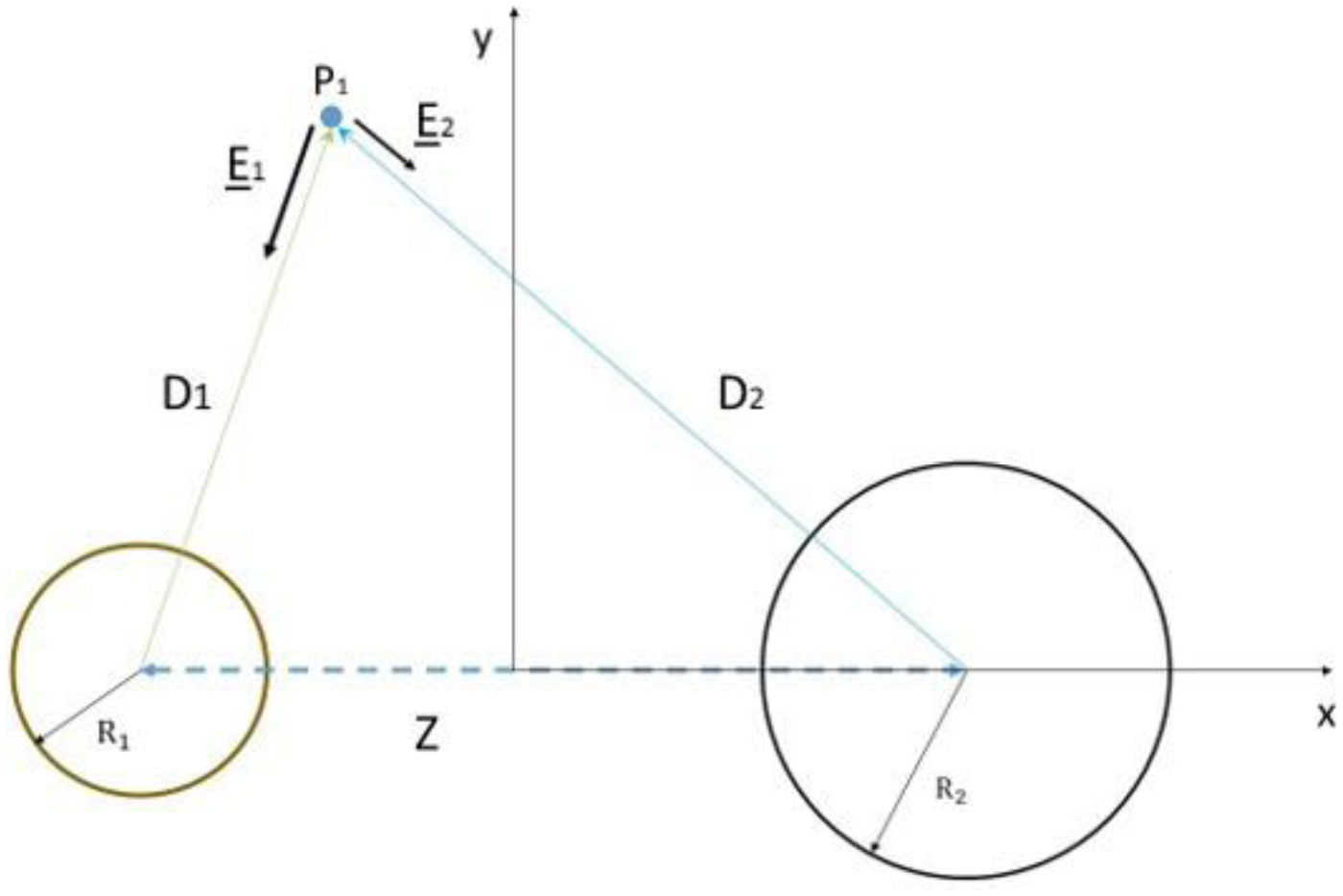
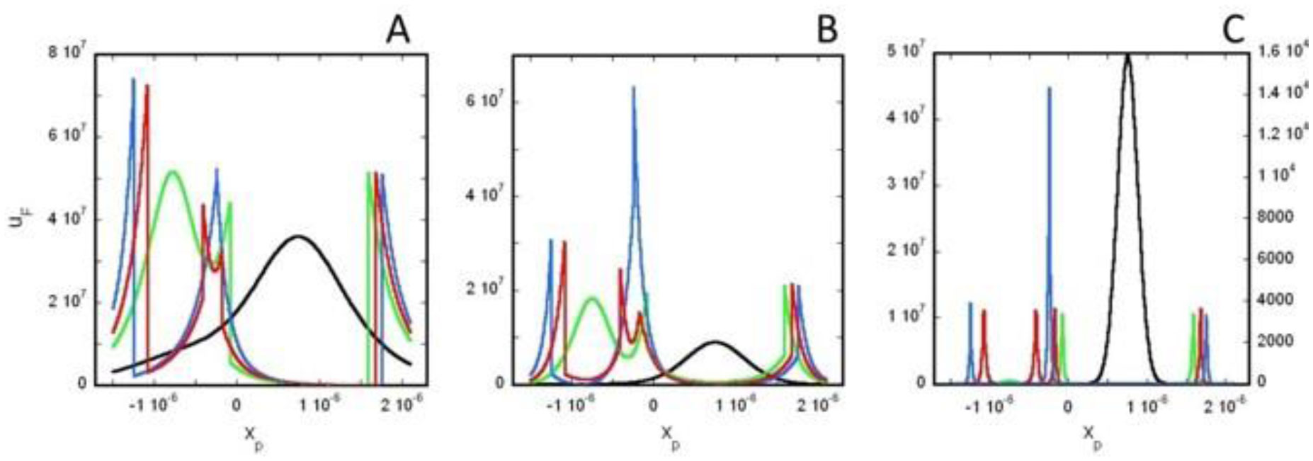
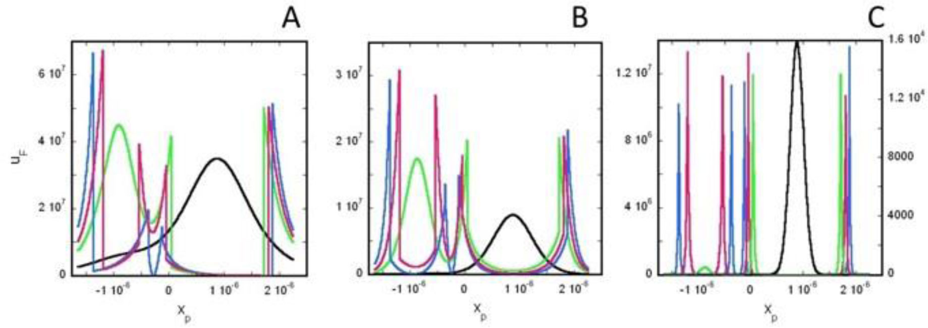
Based on the generalized version of Newton's Shell Theorem the electric field energy density, u_F around two separated surface-charged spheres surrounded by electrolyte is calculated. According to the calculations when the surfaces of the charged spheres are farther from each other than four times of the Debye length the field energy density around one of the charged sphere is basically independent from the presence of the other sphere. In this case at low electrolyte ion concentration u_F = 0 within the spheres and outside the sphere u_F decreases with increasing distance from the surface of the sphere, while at high electrolyte ion concentration u_F fast decreases with increasing inner and outer distance from the surface of the sphere. When the charged sheres are close to each other their electric interaction affects the field energy density especially where the surfaces of the spheres are close to each other. Also to model electrophoresis analytical equations are derived for the interaction energy between and the density of electric field energy around a charged flat surface and a charged sphere surrounded by neutral electrolyte.

Keywords:

Citation: István P. Sugár. Density of electric field energy around two surface-charged spheres surrounded by electrolyte I. The spheres are separated from each other[J]. AIMS Biophysics, 2022, 9(2): 86-95. doi: 10.3934/biophy.2022008

Related Papers:

[1]	István P. Sugár . Density of electric field energy around two surface-charged spheres surrounded by electrolyte II. The smaller sphere is inside the larger one. AIMS Biophysics, 2022, 9(1): 61-71. doi: 10.3934/biophy.2022006
[2]	István P. Sugár . Electric energies of a charged sphere surrounded by electrolyte. AIMS Biophysics, 2021, 8(2): 157-164. doi: 10.3934/biophy.2021012
[3]	István P. Sugár . A generalization of the Shell Theorem. Electric potential of charged spheres and charged vesicles surrounded by electrolyte. AIMS Biophysics, 2020, 7(2): 76-89. doi: 10.3934/biophy.2020007
[4]	István P. Sugár . A generalization of the Shell Theorem. Electric potential of charged spheres and charged vesicles surrounded by electrolyte. AIMS Biophysics, 2023, 10(1): 23-24. doi: 10.3934/biophy.2023003
[5]	Ganesh Prasad Tiwari, Santosh Adhikari, Hari Prasad Lamichhane, Dinesh Kumar Chaudhary . Natural bond orbital analysis of dication magnesium complexes [Mg(H₂O)₆]²⁺ and [[Mg(H₂O)₆](H₂O)_n]²⁺; n=1-4. AIMS Biophysics, 2023, 10(1): 121-131. doi: 10.3934/biophy.2023009
[6]	Hanieh Hadady, Doug Redelman, Sage R. Hiibel, Emil J. Geiger . Continuous-flow sorting of microalgae cells based on lipid content by high frequency dielectrophoresis. AIMS Biophysics, 2016, 3(3): 398-414. doi: 10.3934/biophy.2016.3.398
[7]	Klemen Bohinc, Leo Lue . On the electrostatics of DNA in chromatin. AIMS Biophysics, 2016, 3(1): 75-87. doi: 10.3934/biophy.2016.1.75
[8]	Piotr H. Pawłowski, Piotr Zielenkiewicz . The role of electric charge in SARS-CoV-2 and other viral infections. AIMS Biophysics, 2024, 11(2): 166-188. doi: 10.3934/biophy.2024011
[9]	Massimo Fioranelli, Maria Grazia Roccia, Aroonkumar Beesham, Dana Flavin, M. Ghaeni, Faissal AZIZ . A model for considering effects of extremely low frequency electromagnetic fields on quail embryonic cells. AIMS Biophysics, 2022, 9(3): 198-207. doi: 10.3934/biophy.2022017
[10]	David E. Shoup . Diffusion-controlled reaction rates for clusters of binding sites on a cell. AIMS Biophysics, 2016, 3(4): 522-528. doi: 10.3934/biophy.2016.4.522

Abstract

1. Introduction

The headgroups of membrane lipids have either single charge (e.g. tetraether lipids [1],[2] phosphatidic acid (PA), phosphatidylserine (PS), phosphatidylethanolamine (PE), and phosphatidylinositol (PI)) or electric dipole (e.g. phospholipids [1],[3] like dipalmitoyl-, distearoyl-, dimyristoylphosphatidylcholine). Theoretical models of lipid membranes usually focus on short range (Van der Waals) lateral interactions between nearest neighbor lipids and ignore the long range charge-charge interactions [3],[4]. This is because in the case of long range interactions one has to consider the entire system rather than the interactions between the nearest neighbor lipids. Charges, like head group charges, that are embedded into electrolyte (electroneutral ion solution), but not part of the electrolyte itself, are called external charges. The potential, V, generated by external charges can be calculated by solving the Screened Poisson Equation, ([5] and see Eq 3 in ref. [6] or Eq A17 in Appendix 4).

By using the solution of the Screened Poisson Equation Newton's Shell Theorem was generalized [6],[7] and then it was possible to calculate analytically different electrical properties of one and two concentric surface-charged spheres (surrounded inside and outside by electrolyte) such as: electric energy required to build up the charged sphere(s) [8], electric field energy inside and outside the sphere(s) [8], polarization energy of the electrolyte ions [8] and electric interaction energy between the charged spheres [9].

In this work the density of the electric field energy inside and outside of two charged spheres are calculated at different locations. The density of the electric field energy at a point can be calculated by the following equation [10]:

$u_{F} = \frac{ϵ_{r} ϵ_{0}}{2} \underline{E} \cdot \underline{E}$ (1)

where E is the vector of the electric field strength at the considered point, ϵ₀ is the absolute vacuum permittivity and ϵ_r is the relative permittivity of the electrolyte.

Note that the Poisson-Boltzmann equation [11] can be used to calculate the potential, V of an arbitrary, electroneutral, ion solution (i.e. electrolyte). However, for the solution of the equation one has to know the charge density of the ions in the electrolyte (i.e. the Boltzmann distribution) which depends on the potential, V, itself. Thus, only approximative solution (e.g. Debye-Hückel approximation [11]) is available, that is valid when $| z_{i} e V / (k_{B} T) | ≪ 1$ (where e: charge of an electron, z_i: charge number of the i-th type of ion, k_B: Boltzmann constant, T: absolute temperature). Using the general solution of the Screened Poisson Equation (Eq A17) one can calculate the potential energy of an electrolyte that contains also external charges. The external charges are embedded into the electrolyte (like the charges of the surface-charged sphere) but not part of the electrolyte itself. For the solution one has to know the charge density of the external charges, ρ_ex (see Eq A17), i.e. the distribution of the charges on the surface-charged sphere and not the distribution of the ions in the electrolyte. In our case it is assumed that the charges on the surface of the sphere are homogeneously distributed and in this case one can get the exact solution of the Screened Poisson Equation (see Eqs 9,10 in ref. [6] or Eqs A1, A2 in Appendix 1).

2. Model

By using the generalized Shell Theorem [6] we calculate the density of electric field energy, u_F produced by two surface-charged spheres (see Figure 1) surrounded outside and inside by electrolyte. The surface of each sphere is homogeneously charged. The total charge of the smaller and larger sphere is Q₁ and Q₂, respectively.

Figure 1. Two surface-charged spheres surrounded outside and inside by neutral electrolyte. Z: the distance between the centers of the spheres (dashed blue line); R₁ and R₂ is the radius of the smaller and larger sphere, respectively; D₁ and D₂ is the distance between point P₁ and the center of the smaller and larger sphere, respectively; E₁ and E₂ is the field strength created at point P₁ by the smaller and larger charged sphere, respectively.

DownLoad: Full-Size Img PowerPoint

In Figure 1 the origin of the coordinate system (x, y) is attached to the middle of the distance between the centers of the two spheres, and the coordinates of point P₁ are x_p and y_p. The coordinates of the center of the larger and smaller sphere are $(x_{2}, y_{2}) = (Z / 2, 0)$ and $(x_{1}, y_{1}) = (- Z / 2, 0)$ , respectively.

In order to calculate the density of electric field energy one needs the electric field strength (see Eq 1), i.e. the gradient of the electric potential. The potential produced by the smaller sphere, V₁ can be calculated by Eqs 9,10 in ref. [6] (see also Eqs A1, A2 in Appendix 1) and from the gradient of this potential the electric field strength created by the smaller sphere at point P₁ (see Figure 1) is:

${\underline{E}}_{1} = - g r a d (V_{1}) = - (\frac{d V_{1}}{d D_{1}} \frac{d D_{1}}{d x_{P}}, \frac{d V_{1}}{d D_{1}} \frac{d D_{1}}{d y_{P}}) = - \frac{d V_{1}}{d D_{1}} (\frac{d \sqrt{{(x_{P} - x_{1})}^{2} + {(y_{P} - y_{1})}^{2}}}{d x_{P}}, \frac{d \sqrt{{(x_{P} - x_{1})}^{2} + {(y_{P} - y_{1})}^{2}}}{d y_{P}}) = - \frac{d V_{1}}{d D_{1}} (\frac{x_{P} - x_{1}}{D_{1}}, \frac{y_{P} - y_{1}}{D_{1}}) = (- \frac{d V_{1}}{d D_{1}} \frac{x_{P} + (\frac{Z}{2})}{D_{1}}, - \frac{d V_{1}}{d D_{1}} \frac{y_{P}}{D_{1}}) = (E_{1 x}, E_{1 y})$ (2)

where

$\frac{d V_{1}}{d D_{1}} = {\begin{matrix} \frac{k_{e} Q_{1} λ_{D}}{ϵ_{r} R_{1}} s i n h (R_{1} / λ_{D}) [- \frac{e^{- \frac{D_{1}}{λ_{D}}}}{D_{1}^{2}} - \frac{e^{- \frac{D_{1}}{λ_{D}}}}{D_{1} λ_{D}}] i f D_{1} > R_{1} \\ \frac{k_{e} Q_{1} λ_{D}}{ϵ_{r} R_{1}} e^{- \frac{R_{1}}{λ_{D}}} [- \frac{s i n h (\frac{D_{1}}{λ_{D}})}{D_{1}^{2}} + \frac{c o s h (\frac{D_{1}}{λ_{D}})}{D_{1} λ_{D}}] i f D_{1} < R_{1} \end{matrix}$ (3)

where λ_D is the Debye length (see Eq A3) and $R_{1} + R_{2} < Z$ .

Similarly, the electric field strength created by the larger sphere at point P₁ (see Figure 1) is:

${\underline{E}}_{2} = - g r a d (V_{2}) = - (\frac{d V_{2}}{d D_{2}} \frac{d D_{2}}{d x_{P}}, \frac{d V_{2}}{d D_{2}} \frac{d D_{2}}{d y_{P}}) = - \frac{d V_{2}}{d D_{2}} (\frac{d \sqrt{{(x_{P} - x_{2})}^{2} + {(y_{P} - y_{2})}^{2}}}{d x_{P}}, \frac{d \sqrt{{(x_{P} - x_{2})}^{2} + {(y_{P} - y_{2})}^{2}}}{d y_{P}}) = - \frac{d V_{2}}{d D_{2}} (\frac{x_{P} - x_{2}}{D_{2}}, \frac{y_{P} - y_{2}}{D_{2}}) = (- \frac{d V_{2}}{d D_{2}} \frac{x_{P} - (\frac{Z}{2})}{D_{2}}, - \frac{d V_{2}}{d D_{2}} \frac{y_{P}}{D_{2}}) = (E_{2 x}, E_{2 y})$ (4)

where one can construct dV₂/dD₂ from Eq 3 by substituting D₁ by D₂, R₁ by R₂ and Q₁ by Q₂.

Finally, based on Eq 1 the density of the electric field energy at point P₁ is:

$u_{F} (x_{P}, y_{P}) = \frac{ϵ_{r} ϵ_{0}}{2} \underline{E} \cdot \underline{E} = \frac{ϵ_{r} ϵ_{0}}{2} ({\underline{E}}_{1} + {\underline{E}}_{2}) \cdot ({\underline{E}}_{1} + {\underline{E}}_{2}) = \frac{ϵ_{r} ϵ_{0}}{2} ([E_{1 x} + E_{2 x}], [E_{1 y} + E_{2 y}]) \cdot ([E_{1 x} + E_{2 x}], [E_{1 y} + E_{2 y}]) = \frac{ϵ_{r} ϵ_{0}}{2} ({[E_{1 x} + E_{2 x}]}^{2} + {[E_{1 y} + E_{2 y}]}^{2})$ (5)

3. Results

Figure 2. Locations where electric field energy density around two surface-charged spheres are calculated. A) At the origin of the coordinate system, marked by black dot, two charged spheres of radius R₂ are connected. The distance between their centers is Z = 2 R₂. In Figure 3 the electric field energy densities are calculated along the three horizontal lines. B) Two separated charged spheres of radius R₂. The distance between their centers is Z = 2.5 R₂. In Figure 4 the electric field energy densities are calculated along the three horizontal lines. C) Two charged spheres of radius R₂ and R₁ (= 0.5 R₂) are connected. The distance between their centers is Z = 3 R₁. In Figure 5 the electric field energy densities are calculated along the four horizontal lines. D) Two separated charged spheres of radius R₂ and R₁ (= 0.5 R₂). The distance between their centers is Z = 3.5 R₁. In Figure 6 the electric field energy densities are calculated along the four horizontal lines.

DownLoad: Full-Size Img PowerPoint

Here by using Eq 5 the density of the electric field energy, u_F, is calculated around two surface-charged spheres surrounded in- and outside by electrolyte. The radius of the larger and smaller sphere is: R₂ = 10⁻⁶ m and R₁ = 0.5 R₂, respectively. The surface charge density of the homogeneously charged spheres is $ρ_{s} = - 0.266 C / m^{2}$ (the surface charge density of the PLFE lipid vesicles [1],[2]). The total charge of the larger and the smaller sphere is, $Q_{2} = ρ_{s} 4 π R_{2}^{2} = - 3.3427 \cdot 10^{- 12} C$ and $Q_{1} = ρ_{s} 4 π R_{1}^{2} = - 8.3566 \cdot 10^{- 13} C$ , respectively. This system is axially symmetric, where the symmetry axis is the straight line connecting the centers of the spheres. The center of the attached coordinate system is at the midpoint between the centers of the spheres (see black dots in Figures 2A-D), and the x axis is defined by the symmetry axis. Because of the axial symmetry of the system it is enough to calculate u_F along straight lines parallel to the symmetry axis (see Figure 2), where the same y_P coordinate belongs to each straight line. If the spheres have the same total charge and the same radius (see Figure 2A, B) the system has lateral symmetry too and thus $u_{F} (- x_{P}, y_{P}) = u_{F} (x_{P}, y_{P})$ . The charged spheres are surrounded by neutral electrolyte containing monovalent ions. The considered electrolyte ion concentrations (of the positive ion) are: 0.00001, 0.001 and 0.1mol/m³ and the respective Debye lengths (calculated by Eq A3) are: 3.05 · 10⁻⁶, 3.05 · 10⁻⁷ and 3.05 · 10⁻⁸m, and the relative permittivity of the electrolyte is ϵ_r = 78.

Figure 3. Density of the electric field energy around two connected similarly charged spheres of the same size. Two surface-charged spheres each of radius R₂ are shown in Figure 2A. The distance between their centers is Z = 2 R₂ and the center of the coordinate system is located at the middle of this distance. The electric field energy densities are calculated along the three horizontal lines (shown in Figure 2A): at blue line y_P = 0; at red line y_P = 0.75 R₂; at black line y_P = 1.1 R₂. The concentration of the monovalent positive (or negative) ion in the electrolyte is: A) C = 0.00001mol/m³; B) C = 0.001mol/m³; C) C = 0.1mol/m³. In Figure 3C regarding the black curve the values of u_F are shown on the right side.

DownLoad: Full-Size Img PowerPoint

$x_{p}^{c} = \pm 0.5 Z (1 \pm \sqrt{1 - {(y_{p} / R_{2})}^{2}}) .$ (6)

Figure 4. Density of the electric field energy around two separated similarly charged spheres of the same size. Two separated surface-charged spheres each of radius R₂ are shown in Figure 2B. The distance between their centers is Z = 2.5 R₂ and the center of the coordinate system is located at the middle of this distance. The electric field energy densities are calculated along the three horizontal lines (shown in Figure 2B): at blue line y_P = 0; at red line y_P = 0.75 R₂; at black line y_P = 1.1 R₂. The concentration of the monovalent positive (or negative) ion in the electrolyte is: A) C = 0.00001mol/m³; B) C = 0.001mol/m³; C) C = 0.1mol/m³. In Figure 4C regarding the black curve the values of u_F are shown on the right side.

DownLoad: Full-Size Img PowerPoint

Figure 5. Density of the electric field energy around two connected charged spheres of different sizes. Two surface-charged spheres of radius R₂ and R₁(= 0.5 R₂) are shown in Figure 2C. The distance between their centers is Z = 3 R₁ and the center of the coordinate system is located at the middle of this distance. The electric field energy densities are calculated along the four horizontal lines (shown in Figure 2C): at blue line y_P = 0; at red line y_P = 0.75 R₁; at green line y_P = 1.1 R₁; at black line y_P = 1.1 R₂. The concentration of the monovalent positive (or negative) ion in the electrolyte is: A) C = 0.00001mol/m³; B) C = 0.001mol/m³; C) C = 0.1mol/m³. In Figure 5C regarding the black curve the values of u_F are shown on the right side.

DownLoad: Full-Size Img PowerPoint

The connection point between the spheres of different sizes is at x_P = −0.5 R₁ and y_P = 0. At this point there is no electrolyte and Eqs 2–5 are not applicable. The field energy densities approaching this connection point from left (i.e. x_p → −0.5 R₁₋ where R₁₋ ⪅ R₁; y_p = 0) and from right (i.e. x_p → −0.5 R₁₊ where R₁₊ ⪆ R₁; y_p = 0) are shown by the blue curves in Figures 5A–C. Similar situations take place when the horizontal line crosses the circles (at y_p > 0) in Figure 2C,D. The x_p coordinates of these cross sections, $x_{p}^{c}$ can be calculated by:

$x_{p}^{c} = - 0.5 Z (1 \pm \sqrt{1 - {(y_{p} / R_{1})}^{2}}) at x_{p} < - 0.5 Z + R_{1} and y_{P} < R_{1} .$ (7)

and

$x_{p}^{c} = 0.5 Z (1 \pm \sqrt{1 - {(y_{p} / R_{2})}^{2}}) at x_{p} > - 0.5 Z + R_{1} and y_{P} < R_{2} .$ (8)

Figure 6. Density of the electric field energy around two separated charged spheres of different sizes. Two separated surface-charged spheres of radius R₂ and R₁(= 0.5 R₂) are shown in Figure 2D. The distance between their centers is Z = 3.5 R₁ and the center of the coordinate system is located at the middle of this distance. The electric field energy densities are calculated along the four horizontal lines (shown in Figure 2D): at blue line y_P = 0; at red line y_P = 0.75 R₁; at green line y_P = 1.1 R₁; at black line y_P = 1.1 R₂. The concentration of the monovalent positive (or negative) ion in the electrolyte is: A) C = 0.00001mol/m³; B) C = 0.001mol/m³; C) C = 0.1mol/m³. In Figure 6C regarding the black curve the values of u_F are shown on the right side.

DownLoad: Full-Size Img PowerPoint

4. Discussion

The density of the electric field energy depends on the electric field strength (Eq 1), i.e. the gradient of the electric potential. In the case of a single charged sphere surrounded by electrolyte with low ion concentration the potential inside the sphere is close to constant (see red curve in Figure 3A in ref. [6]) and thus the absolute value of the electric field strength is close to zero. On the other hand, outside the sphere the absolute value of the potential and also the electric field strength decrease with increasing distance from the surface of the sphere (see red curve in Figure 3A in ref. [6]). At higher electrolyte ion concentration, because of the increased screening effect, the absolute value of the potential and also the electric field strength decrease faster with increasing distance from the surface of the sphere. In this case inside the sphere toward its center the absolute value of the potential and the electric field strength also decrease (see curves in Figure 3A,B in ref. [6]).

These electric properties of a single charged sphere remain unchanged in the case of two charged spheres if the surfaces of the spheres are far enough from each other (farther than 4λ_D), i.e. the potential of one of the sphere decreases close to zero near the surface of the other sphere. However, when the two spheres are close enough to each other one sphere contributes to the potential and electric field strength around the other sphere. For example, let us consider two spheres of the same size located close to each other (see the left and right sphere in Figure 2B) and the electrolyte ion concentration is very low (C = 0.00001mol/m³). In this case the charges of the left sphere create close to zero electric field strength inside the left sphere, while the electric field strength created outside of the right sphere (by the charges of the right sphere) decreases toward the left sphere and further decreases inside the left sphere. Thus, within the left sphere on its right side u_F is rather high (see Figure 4A blue line at $x_{P} < - 0.25 \cdot 10^{- 6} m$ ) while it is close to zero on its left side. However, crossing the left surface of the left sphere u_F jumps up because the field strength jumps from close to zero to $| {\underline{E}}_{1} | ≅ k_{e} Q_{1} / ϵ_{r} R_{1}^{2}$ (see Figure 4A blue line at $x_{P} = - 2.25 \cdot 10^{- 6} m$ ). In general, when the horizontal line crosses the sphere(s) (see Figure 2) u_F has sharp maxima (see Figures 3–6). When the horizontal line does not cross the spheres of the same size (i.e. y_p > R₂) u_F has two broad maxima where the distance between the horizontal line and the surface of the spheres is minimal (see black curves in Figures 3,4). However, when the sizes of the two spheres are different the maximum of u_F close to the larger sphere is larger than the other maximum (close to the smaller sphere). These maxima are broader when the electrolyte ion concentration is low. In this case the smaller maximum may disappear because the larger one overlaps the smaller one (see black line in Figures 5A and 6A).

At the midpoint between the two separated spheres of the same size (at x_P = 0 and y_P = 0) u_F = 0 J m⁻³ because at the symmetry center the absolute value of electric field created by the left sphere is equal with the absolute value of electric field created by the right sphere, but their direction is opposite (thus $E_{1 x} + E_{2 x} = 0$ while $E_{1 y} = E_{2 y} = 0$ ). Approaching from the midpoint the outer surface of the left sphere u_F increases, but the increase is slower than in the case of a single sphere because the presence of the right sphere (with opposite direction its electric field vector) reduces the outer electric field strength of the left sphere.

At x_P = 0 and $y_{P} > 0 u_{F} > 0 J m^{- 3}$ because $E_{1 y} = E_{2 y} \neq 0$ and thus ${[E_{1 y} + E_{2 y}]}^{2} > 0$ (see Figure 4A red and black line). With increasing electrolyte ion concentration as a consequence of the increasing screening ${[E_{1 y} + E_{2 y}]}^{2}$ is getting smaller and thus u_F is getting smaller too (compare Figure 4A, B and C at x_P = 0 and at the same y_P).

The connection point between the spheres of the same size is at x_P = 0 and y_P = 0 (see black dot in Figure 2A). At this point there is no electrolyte and Eqs 2–5 are not applicable. The field energy densities approaching this connection point from left (i.e. x_p → 0₋; y_p = 0) and from right (i.e. x_p → 0₊; y_p = 0) are shown by the blue curves in Figures 3A–C. It is pointed out in Appendix 2 that, at any electrolyte ion concentration, in the case of R₁ = R₂ the density of the field energy is the same either approaching the connection point from the left or right (see Eqs A5, A7). However, if the right sphere is larger than the left sphere (i.e. R₂ > R₁) then u_F near the right side of the connection point is larger than u_F near the left side of the connection point (see Eqs A8, A9). Note, that the difference between these field energy densities decreases with decreasing electrolyte ion concentration and the difference becomes zero at zero electrolyte ion concentration (see Eqs A12, A13).

The analytical equation for the calculation of the electric field energy density of two charged spheres, Eq 5 is generalized for N charged spheres in Appendix 3.

In this paper two surface-charged spheres surrounded by electrolyte is considered. This system is close to the case of electrophoresis where charged cells surrounded by electrolyte interact with a charged flat surface [12],[13]. In Appendix 4 analytical equations are derived for this kind of system by using the solution of the Screened Poisson Equation (see Eq 4 in ref. [6]). The density of electric field energy around a charged sphere and a charged flat surface can be calculated at point (x_p, y_p) [see Fig.A1(B)] by Eq 5 where E₁ is given by Eqs 2,3 and ${\underline{E}}_{2} = (E_{2 x}, E_{2 y})$ is given at Eq A24:

$(E_{2 x}, E_{2 y}) = (- \frac{ρ_{2}}{2 ϵ_{o} ϵ_{r}} e^{- \frac{0.5 Z - x_{p}}{λ_{D}}}, 0)$ (9)

5. Conclusions

Based on the generalized version of Newton's Shell Theorem [6] analytical equation is derived to calculate the electric field energy density, u_F around two separated surface-charged spheres surrounded by electrolyte. According to the calculations when the surfaces of the charged spheres are farther from each other than four times of the Debye length the field energy density around one of the charged sphere is basically independent from the presence of the other sphere. In this case at low electrolyte ion concentration u_F = 0 within the spheres and outside the sphere u_F decreases with increasing distance from the surface of the sphere, while at high electrolyte ion concentration u_F fast decreases with increasing inner and outer distance from the surface of the sphere. When the charged spheres are close to each other their electric interaction affects the field energy density especially where the surfaces of the spheres are close to each other. Also, to model electrophoresis analytical equations are derived for the interaction energy between and the density of electric field energy around a charged flat surface and a surface-charged sphere surrounded by neutral electrolyte.

Acknowledgments

The author is very thankful for Chinmoy Kumar Ghose.

Conflict of interest

The author declares no conflict of interest.

References

[1]	Gabriel JL, Chong PLG (2000) Molecular modeling of archaebacterial bipolar tetraether lipid membranes. Chem Phys Lipids 105: 193-200. https://doi.org/10.1016/S0009-3084(00)00126-2
[2]	Chong PLG (2010) Archaebacterial bipolar tetraether lipids: Physico-chemical and membrane properties. Chem Phys Lipids 163: 253-265. https://doi.org/10.1016/j.chemphyslip.2009.12.006
[3]	Almeida PFF (2009) Thermodynamics of lipid interactions in complex bilayers. BBA-Biomembranes 1788: 72-85. https://doi.org/10.1016/j.bbamem.2008.08.007
[4]	Sugár IP, Thompson TE, Biltonen RL (1999) Monte Carlo simulation of two-component bilayers: DMPC/DSPC mixtures. Biophys J 76: 2099-2110. https://doi.org/10.1016/S0006-3495(99)77366-2
[5]	Fetter AL, Walecka JD (2003) Theoretical Mechanics of Particles and Continua. New York: Dover Publications 307-310.
[6]	Sugár IP (2020) A generalization of the shell theorem. Electric potential of charged spheres and charged vesicles surrounded by electrolyte. AIMS Biophys 7: 76-89. https://doi.org/10.3934/biophy.2020007
[7]	Newton I (1999) The Principia: Mathematical Principles of Natural Philosophy. Berkeley: University of California Press.
[8]	Sugár IP (2021) Electric energies of a charged sphere surrounded by electrolyte. AIMS Biophys 8: 157-164. https://doi.org/10.3934/biophy.2021012
[9]	Sugár IP (2021) Interaction energy between two separated charged spheres surrounded inside and outside by electrolyte. arXiv:2103.13959 .
[10]	Griffiths DJ (2005) Introduction to electrodynamics. AM J Phys 73: 574. https://doi.org/10.1119/1.4766311
[11]	Holtzer AM (1954) The collected papers of Peter JW Debye. Interscience, New York-London, 1954. xxi+ 700 pp., $9.50. J Polym Sci 13: 548-548. https://doi.org/10.1002/pol.1954.120137203
[12]	Levin S, Levin M, Sharp AK, et al. (1983) Theory of electrokinetic behavior of human erythrocytes. Biophys J 42: 127-135. https://doi.org/10.1016/S0006-3495(83)84378-1
[13]	Korohoda W, Wilk A (2008) Cell Electrophoreses–a method for cell separation and research into cell surface properties. Cell Mol Biol Lett 18: 312-326. https://doi.org/10.2478/s11658-008-0004-y

biophy-09-02-008-s001.pdf

Reader Comments

Your name:*

Email:*
© 2022 the Author(s), licensee AIMS Press. This is an open access article distributed under the terms of the Creative Commons Attribution License (http://creativecommons.org/licenses/by/4.0)

通讯作者: 陈斌, bchen63@163.com

1.
沈阳化工大学材料科学与工程学院沈阳 110142

AIMS Biophysics

1.1 2.4

Metrics

Article views(1725) PDF downloads(180) Cited by(0)

Preview PDF

Download XML

Export Citation

Article outline

Show full outline

Figures and Tables

Figures(6)

AIMS Biophysics

Density of electric field energy around two surface-charged spheres surrounded by electrolyte I. The spheres are separated from each other

Related Papers:

Abstract

1. Introduction

2. Model

3. Results

4. Discussion

5. Conclusions

References

Reader Comments

通讯作者: 陈斌, bchen63@163.com

Metrics

Figures and Tables

Other Articles By Authors

Catalog

AIMS Biophysics

Density of electric field energy around two surface-charged spheres surrounded by electrolyte I. The spheres are separated from each other

Related Papers:

Abstract

1. Introduction

2. Model

3. Results

4. Discussion

5. Conclusions

References

Reader Comments

通讯作者: 陈斌, bchen63@163.com

Metrics

Figures and Tables

Other Articles By Authors

Related pages

Tools

Export File

Citation

Format

Content

Catalog