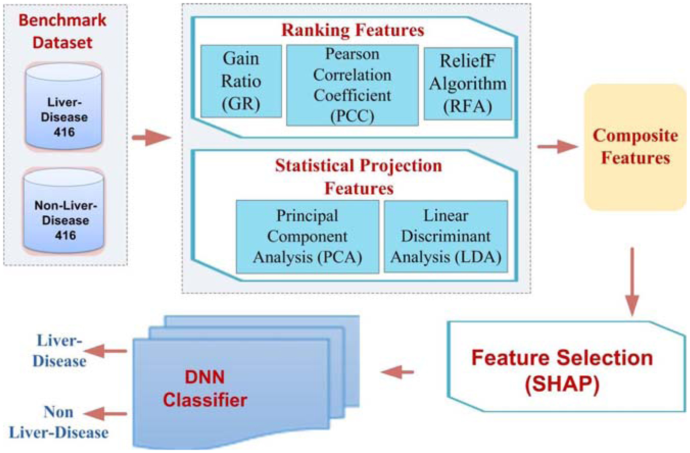
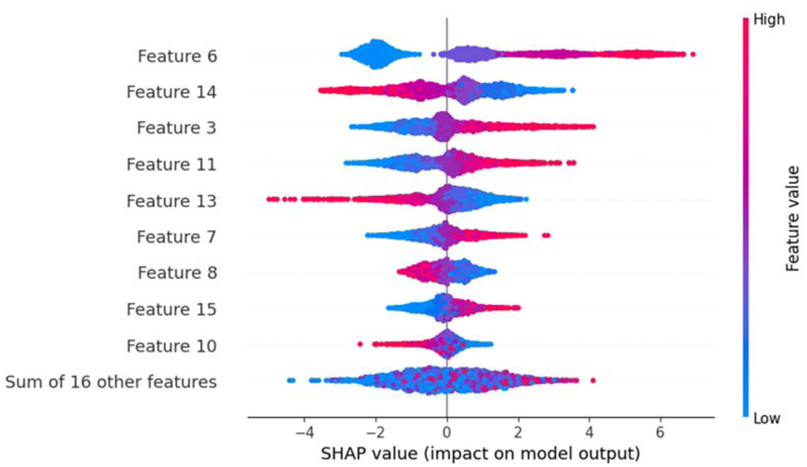
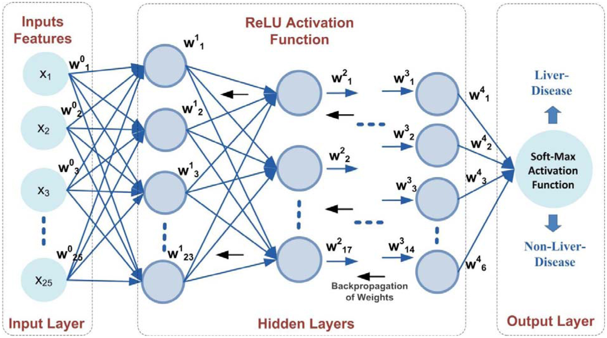
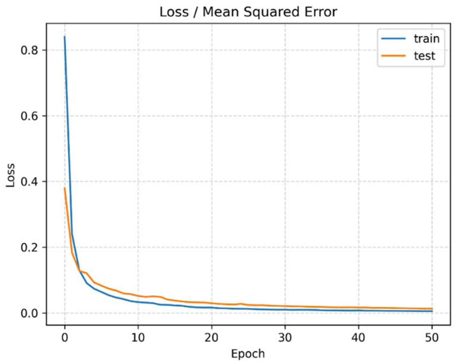
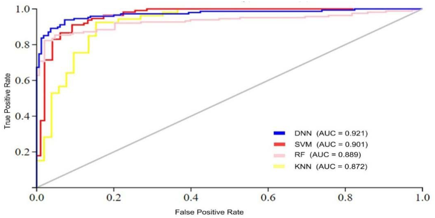
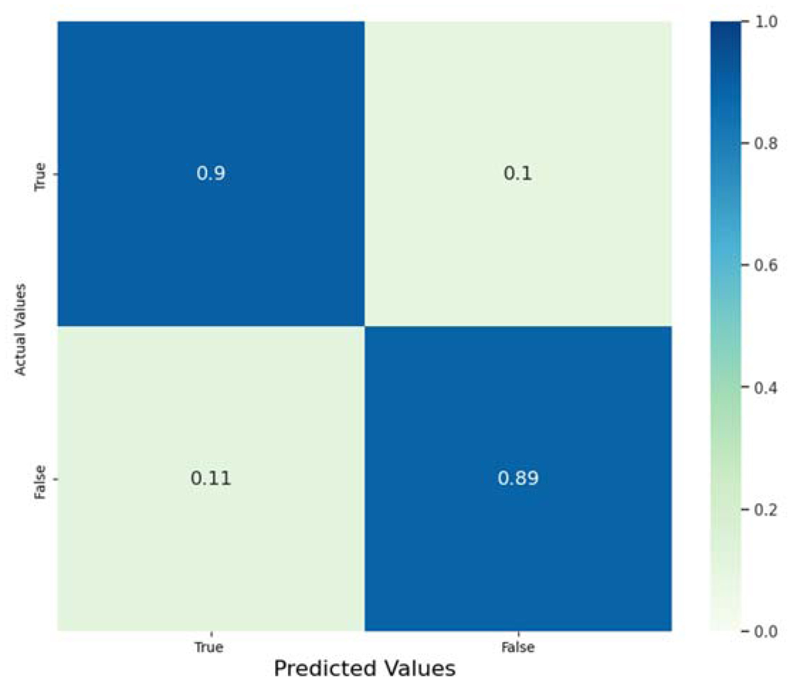
The liver is a vital gland responsible for various essential functions such as digestion, metabolism, detoxification, and immunity. Liver diseases caused by infections, injuries, or genetic factors are dangerous and require prompt diagnosis and treatment to improve survival rates. Early detection of liver conditions is crucial, and recent advancements in machine learning (ML) have proven highly effective in predicting diseases like chronic obstructive pulmonary disease (COPD), hypertension, and diabetes. Additionally, the rise of deep learning has begun transforming liver research, offering powerful tools to aid doctors in diagnosis and treatment. This study presents a novel and efficient learning method to identify liver patients accurately. The approach integrates multiple ranking and projection techniques for features, utilizing deep learning to detect early signs of liver disease. Additionally, Shapley Additive exPlanations (SHAP) are applied to perform global interpretation analysis, helping to select optimal features by assessing their contributions to the overall model. Our experimental results demonstrate that this proposed model outperforms traditional machine learning algorithms, achieving superior accuracy. Cross-validation and various testing methods confirm that the deep neural network (DNN) we developed surpasses other classifiers, reaching an accuracy rate of 90.12%. This paper explores how machine learning can be integrated into healthcare, particularly for predicting liver disease. Our findings show that the proposed model can potentially improve diagnostic accuracy and support timely medical intervention, ultimately enhancing patient outcomes.
Citation: Sumaiya Noor, Salman A. AlQahtani, Salman Khan. Chronic liver disease detection using ranking and projection-based feature optimization with deep learning[J]. AIMS Bioengineering, 2025, 12(1): 50-68. doi: 10.3934/bioeng.2025003
The liver is a vital gland responsible for various essential functions such as digestion, metabolism, detoxification, and immunity. Liver diseases caused by infections, injuries, or genetic factors are dangerous and require prompt diagnosis and treatment to improve survival rates. Early detection of liver conditions is crucial, and recent advancements in machine learning (ML) have proven highly effective in predicting diseases like chronic obstructive pulmonary disease (COPD), hypertension, and diabetes. Additionally, the rise of deep learning has begun transforming liver research, offering powerful tools to aid doctors in diagnosis and treatment. This study presents a novel and efficient learning method to identify liver patients accurately. The approach integrates multiple ranking and projection techniques for features, utilizing deep learning to detect early signs of liver disease. Additionally, Shapley Additive exPlanations (SHAP) are applied to perform global interpretation analysis, helping to select optimal features by assessing their contributions to the overall model. Our experimental results demonstrate that this proposed model outperforms traditional machine learning algorithms, achieving superior accuracy. Cross-validation and various testing methods confirm that the deep neural network (DNN) we developed surpasses other classifiers, reaching an accuracy rate of 90.12%. This paper explores how machine learning can be integrated into healthcare, particularly for predicting liver disease. Our findings show that the proposed model can potentially improve diagnostic accuracy and support timely medical intervention, ultimately enhancing patient outcomes.

| [1] | Singh HR, Rabi S (2019) Study of morphological variations of liver in human. Transl Res Anat 14: 1-5. https://doi.org/10.1016/j.tria.2018.11.004 |
| [2] |
Razavi H (2020) Global epidemiology of viral hepatitis. Gastroenterol Clin North Am 49: 179-189. https://doi.org/10.1016/j.gtc.2020.01.001 
|
| [3] | Miao JH, Miao KH (2018) Cardiotocographic diagnosis of fetal health based on multiclass morphologic pattern predictions using deep learning classification. Int J Adv Comput Sc 9: 1-11. https://doi.org/10.14569/IJACSA.2018.090501 |
| [4] |
Dritsas E, Alexiou S, Moustakas K (2022) COPD severity prediction in elderly with ML techniques. Proceedings of the 15th International Conference on PErvasive Technologies Related to Assistive Environments 2022: 185-189. https://doi.org/10.1145/3529190.3534748
|
| [5] |
Babu MSP, Ramjee M, Katta S, et al. (2016) Implementation of partitional clustering on ILPD dataset to predict liver disorders. 2016 7th IEEE International Conference on Software Engineering and Service Science (ICSESS) . IEEE 1094-1097. https://doi.org/10.1109/ICSESS.2016.7883256
|
| [6] |
Gan D, Shen J, An B, et al. (2020) Integrating TANBN with cost sensitive classification algorithm for imbalanced data in medical diagnosis. Comput Ind Eng 140: 106266. https://doi.org/10.1016/j.cie.2019.106266
|
| [7] |
Anagaw A, Chang YL (2019) A new complement naïve Bayesian approach for biomedical data classification. J Amb Intel Hum Comp 10: 3889-3897. https://doi.org/10.1007/s12652-018-1160-1
|
| [8] |
Sreejith S, Nehemiah HK, Kannan A (2020) Clinical data classification using an enhanced SMOTE and chaotic evolutionary feature selection. Comput Biol Med 126: 103991. https://doi.org/10.1016/j.compbiomed.2020.103991
|
| [9] |
Kuzhippallil MA, Joseph C, Kannan A (2020) Comparative analysis of machine learning techniques for indian liver disease patients. 2020 6th International Conference on Advanced Computing and Communication Systems (ICACCS) . IEEE 778-782. https://doi.org/10.1109/ICACCS48705.2020.9074368
|
| [10] |
Amin R, Yasmin R, Ruhi S, et al. (2023) Prediction of chronic liver disease patients using integrated projection based statistical feature extraction with machine learning algorithms. Informatics in Medicine Unlocked 36: 101155. https://doi.org/10.1016/j.imu.2022.101155
|
| [11] |
Yousefian-Jazi A, Ryu JH, Yoon S, et al. (2014) Decision support in machine vision system for monitoring of TFT-LCD glass substrates manufacturing. J Process Contr 24: 1015-1023. https://doi.org/10.1016/j.jprocont.2013.12.009
|
| [12] |
Jain D, Singh V (2018) Feature selection and classification systems for chronic disease prediction: a review. Egypt Inform J 19: 179-189. https://doi.org/10.1016/j.eij.2018.03.002
|
| [13] |
Khan S, AlQahtani SA, Noor S, et al. (2024) PSSM-Sumo: deep learning based intelligent model for prediction of sumoylation sites using discriminative features. BMC Bioinformatics 25: 284. https://doi.org/10.1186/s12859-024-05917-0
|
| [14] |
Khan S, Khan M, Iqbal N, et al. (2023) Enhancing sumoylation site prediction: a deep neural network with discriminative features. Life 13: 2153. https://doi.org/10.3390/life13112153
|
| [15] |
Naeem M, Qiyas M (2023) Deep intelligent predictive model for the identification of diabetes. AIMS Math 8: 16446-16462. https://doi.org/10.3934/math.2023840
|
| [16] |
Lu J, Kerns RT, Peddada SD, et al. (2011) Principal component analysis-based filtering improves detection for Affymetrix gene expression arrays. Nucleic Acids Res 39: e86-e86. https://doi.org/10.1093/nar/gkr241
|
| [17] |
Heuillet A, Couthouis F, Díaz-Rodríguez N (2022) Collective explainable AI: Explaining cooperative strategies and agent contribution in multiagent reinforcement learning with shapley values. IEEE Comput Intell M 17: 59-71. https://doi.org/10.1109/MCI.2021.3129959
|
| [18] | Khan S, Khan M, Iqbal N, et al. (2022) Deep-PiRNA: Bi-layered prediction model for PIWI-interacting RNA using discriminative features. Comput Mater Contin 72: 2243-2258. https://doi.org/10.32604/cmc.2022.022901 |
| [19] |
Uddin I, Awan HH, Khalid M, et al. (2024) A hybrid residue based sequential encoding mechanism with XGBoost improved ensemble model for identifying 5-hydroxymethylcytosine modifications. Sci Rep 14: 20819. https://doi.org/10.1038/s41598-024-71568-z
|
| [20] |
Bibi N, Khan M, Khan S, et al. (2024) Sequence-Based intelligent model for identification of tumor t cell antigens using fusion features. IEEE Access 12: 155040-155051. https://doi.org/10.1109/ACCESS.2024.3481244
|
| [21] |
Noor S, Naseem A, Awan HH, et al. (2024) Deep-m5U: a deep learning-based approach for RNA 5-methyluridine modification prediction using optimized feature integration. BMC Bioinformatics 25: 360. https://doi.org/10.1186/s12859-024-05978-1
|
| [22] |
Khan S, Khan MA, Khan M, et al. (2023) Optimized feature learning for anti-inflammatory peptide prediction using parallel distributed computing. Appl Sci 13: 7059. https://doi.org/10.3390/app13127059
|
| [23] |
Fawagreh K, Gaber MM, Elyan E (2014) Random forests: from early developments to recent advancements. Syst Sci Control Eng 2: 602-609. https://doi.org/10.1080/21642583.2014.956265
|
| [24] |
Yue S, Li P, Hao P (2003) SVM classification: Its contents and challenges. Appl Math 18: 332-342. https://doi.org/10.1007/s11766-003-0059-5
|
| [25] |
Cheng D, Zhang S, Deng Z, et al. (2014) k NN algorithm with data-driven k value. Advanced Data Mining and Applications: 10th International Conference . Guilin, China: 499-512.
|
| [26] |
Khan S, Uddin I, Khan M, et al. (2024) Sequence based model using deep neural network and hybrid features for identification of 5-hydroxymethylcytosine modification. Sci Rep 14: 9116. https://doi.org/10.1038/s41598-024-59777-y
|
| [27] |
Basit A, Fawwad A, Qureshi H, et al. (2018) Prevalence of diabetes, pre-diabetes and associated risk factors: second National Diabetes Survey of Pakistan (NDSP), 2016–2017. BMJ Open 8: e020961. https://doi.org/10.1136/bmjopen-2017-020961
|
| [28] |
Altaf I, Butt MA, Zaman M (2022) Hard voting meta classifier for disease diagnosis using mean decrease in impurity for tree models. Rev Comput Eng Res 9: 71-82. https://doi.org/10.18488/76.v9i2.3037
|
| [29] | Gupta K, Jiwani N, Afreen N, et al. (2022) Liver disease prediction using machine learning classification techniques. 2022 IEEE 11th International Conference on Communication Systems and Network Technologies (CSNT) . IEEE 221-226. https://doi.org/10.1109/CSNT54456.2022.9787574 |
| [30] |
Dritsas E, Trigka M (2023) Supervised machine learning models for liver disease risk prediction. Computers 12: 19. https://doi.org/10.3390/computers12010019
|
Figures(6) / Tables(9)

Sumaiya Noor, Salman A. AlQahtani, Salman Khan. Chronic liver disease detection using ranking and projection-based feature optimization with deep learning[J]. AIMS Bioengineering, 2025, 12(1): 50-68. doi: 10.3934/bioeng.2025003


 DownLoad: