On the fractional Kelvin-Voigt oscillator

Jayme Vaz Jr.; Edmundo Capelas de Oliveira; Jayme Vaz Jr.; Edmundo Capelas de Oliveira

doi:10.3934/mine.2022006

Mathematics in Engineering

2022, Volume 4, Issue 1: 1-23. doi: 10.3934/mine.2022006

Previous Article Next Article

Research article

On the fractional Kelvin-Voigt oscillator

Departamento de Matemática Aplicada, Universidade Estadual de Campinas, 13083-859 Campinas, SP, Brazil

Received: 08 February 2021 Accepted: 27 April 2021 Published: 02 June 2021

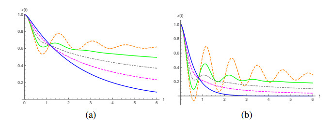
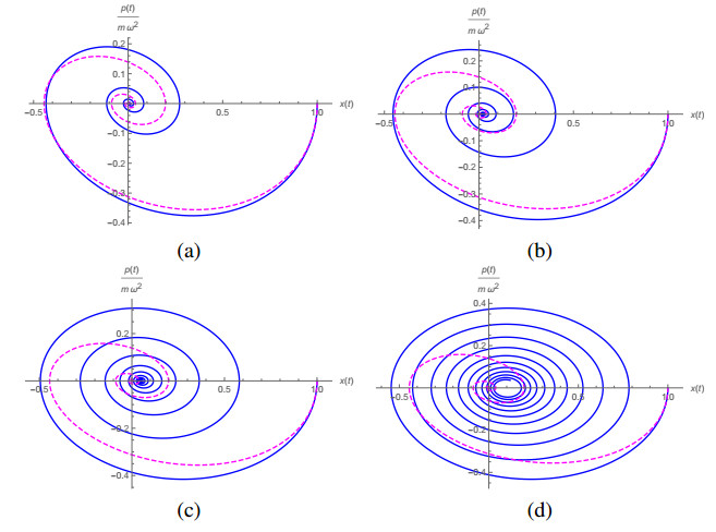
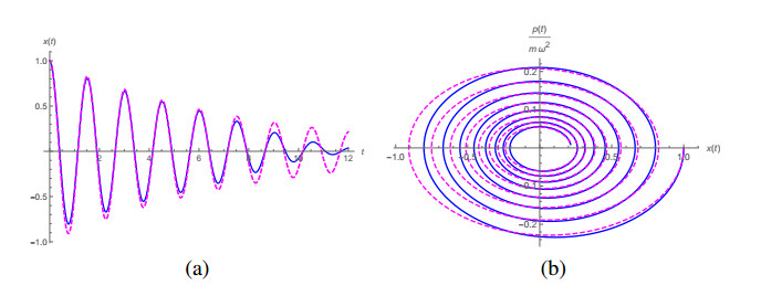
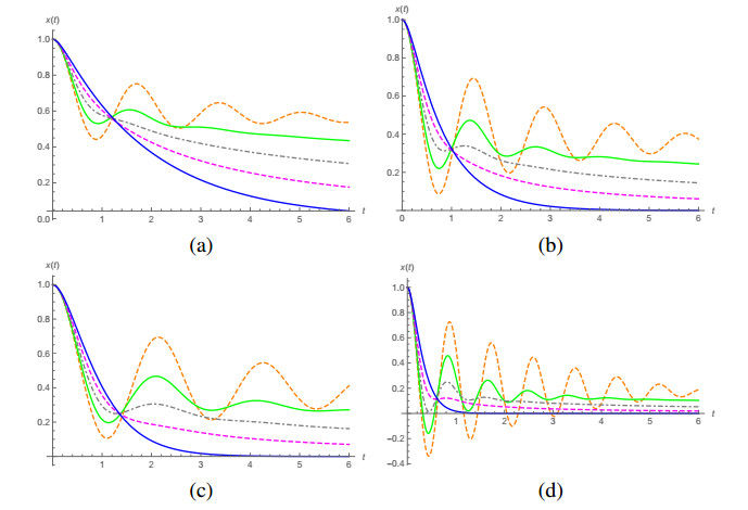
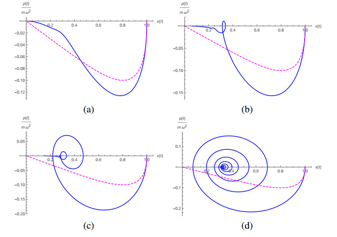
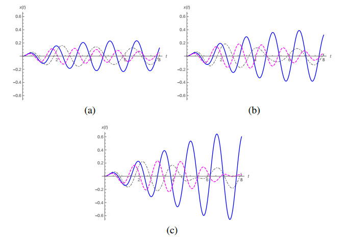
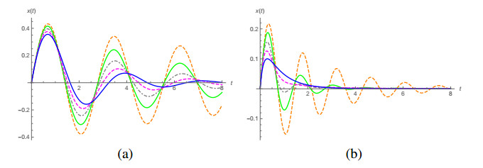
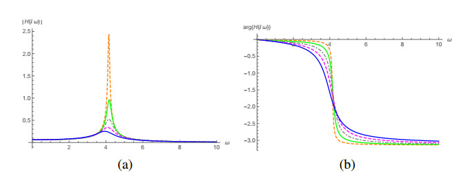
In this paper we discuss the model of fractional oscillator where the inertial and restoring force terms maintains their usual expression but the damping term involves a fractional derivative of Caputo type, the so called fractional Kelvin-Voigt oscillator. The transient solution of this model is given in terms of the so called bivariate Mittag-Leffler function, while the steady-state solution in response to a sinusoidal force involves a 4-variate Mittag-Leffler function. We give numerical examples comparing the solutions for different values of the order $ \alpha $ of the fractional derivative ($ 0 < \alpha \leq 1 $), and compare them with the usual $ \alpha = 1 $ solutions in the underdamped, overdamped and critically damped situations.
- fractional calculus,
- Kelvin-Voigt oscillator,
- Caputo fractional derivative,
- Mittag-Leffler function,
- multivariate Mittag-Leffler function
Citation: Jayme Vaz Jr., Edmundo Capelas de Oliveira. On the fractional Kelvin-Voigt oscillator[J]. Mathematics in Engineering, 2022, 4(1): 1-23. doi: 10.3934/mine.2022006

Related Papers:

Abstract

In this paper we discuss the model of fractional oscillator where the inertial and restoring force terms maintains their usual expression but the damping term involves a fractional derivative of Caputo type, the so called fractional Kelvin-Voigt oscillator. The transient solution of this model is given in terms of the so called bivariate Mittag-Leffler function, while the steady-state solution in response to a sinusoidal force involves a 4-variate Mittag-Leffler function. We give numerical examples comparing the solutions for different values of the order $ \alpha $ of the fractional derivative ($ 0 < \alpha \leq 1 $), and compare them with the usual $ \alpha = 1 $ solutions in the underdamped, overdamped and critically damped situations.

References

[1]	K. B. Oldham, J. Spanier, Fractional calculus: theory and applications of differentiation and integration to arbitrary order, Dover Publications Inc., 2006.
[2]	R. Herrmann, Fractional calculus: an introduction for physicists, 3 Eds., World Scientific Publishing Co, 2018.
[3]	M. M. Merrschaert, A. Sikorskii, Stochastic and computational models for fractional calculus, 2 Eds., de Gruyter, 2019.
[4]	E. C. de Oliveira, Solved exercises in fractional calculus, Switzerland: Springer Nature, 2019.
[5]	I. Podlubny, Fractional differential equations, Academic Press, 1998.
[6]	A. A. Kilbas, H. M. Srivastava, J. J. Trujillo, Theory and applications of fractional differential equations, Elsevier, 2006.
[7]	A. Kochubei, Y. Luchko, Handbook of fractional calculus with applications – Volume 2: fractional differential equations, De Gruyter, 2019.
[8]	F. Mainardi, Fractional relaxation-oscillation and fractional diffusion-wave phenomena, Chaos Soliton. Fract., 7 (1996), 1461–1477. doi: 10.1016/0960-0779(95)00125-5
[9]	B. N. Narahari Achar, J. W. Hanneken, T. Enck, T. Clarke, Dynamics of the fractional oscillator, Physica A, 297 (2001), 361–367. doi: 10.1016/S0378-4371(01)00200-X
[10]	Ya. E. Ryabov, A. Puzenko, Damped oscillations in view of the fractional oscillator equation, Phys. Rev. B, 66 (2002), 184201. doi: 10.1103/PhysRevB.66.184201
[11]	A. A. Stanislavsky, Fractional oscillators, Phys. Rev. E, 70 (2004), 051103.
[12]	Yu. A. Rossikhin, M. V. Shitikova, New approach for the analysis of damped vibrations of fractional oscillators, Shock Vib., 16 (2009), 387676.
[13]	S. S. Ray, S. Sahoo, S. Das, Formulation and solutions of fractional continuously variable order mass–spring–damper systems controlled by viscoelastic and viscous–viscoelastic dampers, Adv. Mech. Eng., 8 (2016), 1–13.
[14]	M. Berman, L. S. Cederbaum, Fractional driven-damped oscillator and its general closed form exact solution, Physica A, 505 (2018), 744–762. doi: 10.1016/j.physa.2018.03.044
[15]	R. Parovik, Mathematical modeling of linear fractional oscillators, Mathematics, 8 (2020), 1879. doi: 10.3390/math8111879
[16]	M. Li, Three classes of fractional oscillators, Symmetry, 10 (2018), 40. doi: 10.3390/sym10020040
[17]	Yu. A. Rossikhin, M. V. Shitikova, Application of fractional calculus for dynamic problems of solid mechanics: novel trends and recent results, Appl. Mech. Rev., 63 (2010), 010801. doi: 10.1115/1.4000563
[18]	Yu. A. Rossikhin, M. V. Shitikova, Application of fractional derivatives on the analysis of damped vibrations of viscoelastic single mass systems, Acta Mech., 120 (1997), 109–125. doi: 10.1007/BF01174319
[19]	R. M. Christensen, Theory of viscoelasticity, 2 Eds., Academic Press Inc., 1982.
[20]	F. Mainardi, Fractional calculus and waves in linear viscoelasticity: an introduction to mathematical models, Imperial College Press, 2010.
[21]	R. L. Bagley, P. J. Torvik, A theoretical basis for the application of fractional calculus to viscoelasticity, J. Rheol., 21 (1983), 201–207.
[22]	R. L. Bagley, P. J. Torvik, On the fractional calculus model of viscoelastic behaviour, J. Rheol., 30 (1986), 133–155. doi: 10.1122/1.549887
[23]	F. Mainardi, R. Gorenflo, Time-fractional derivatives in relaxation processes: a tutorial survey, Fract. Calc. Appl. Anal., 10 (2007), 269–308.
[24]	M. Di Paola, A. Pirrotta, A. Valenza, Visco-elastic behavior through fractional calculus: An easier method for best fitting experimental results, Mech. Mater., 43 (2011), 799–806. doi: 10.1016/j.mechmat.2011.08.016
[25]	E. C. de Oliveira, J. A. Tenreiro Machado, A review of definitions for fractional derivatives and integral, Math. Probl. Eng., 2014 (2014), 238459.
[26]	G. S. Teodoro, J. A. Tenreiro Machado, E. C. de Oliveira, A review of definitions of fractional derivatives and other operators, J. Comput. Phys., 388 (2019), 195–208. doi: 10.1016/j.jcp.2019.03.008
[27]	E. C. de Oliveira, S. Jarosz, J. Vaz Jr., Fractional calculus via Laplace transform and its application in relaxation processes, Commun. Nonlinear Sci., 69 (2019), 58–72. doi: 10.1016/j.cnsns.2018.09.013
[28]	R. Gorenflo, A. A. Kilbas, F. Mainardi, S. Rogosin, Mittag-Leffler functions, related topics and applications, 2 Eds., Springer-Verlag GmbH Germany, 2020.
[29]	H. J. Haubold, A. M. Mathai, R. X. Saxena, Mittag-Leffler functions and their applications, J. Appl. Math., 2011 (2011), 298628.
[30]	G. B. Arfken, H. J. Weber, Mathematical methods for physicists, 6 Eds., Elsevier Science, 2006.
[31]	A. L. Soubhia, R. F. Camargo, E. C. de Oliveira, J. Vaz Jr., Theorem for series in three-parameter Mittag-Leffler function, Fract. Calc. Appl. Anal., 13 (2010), 9–20.
[32]	A. P. Prudnikov, Yu. A. Brychkov, O. I. Marichev, Integrals and series – Volume 1: elementary functions, Gordon and Breach, 1986.
[33]	A. H. Zemanian, Distribution theory and transform analysis: an introduction to generalized functions, with applications, Dover Publications Inc., 2010.
[34]	R. P. Kanwal, Generalized functions: theory and applications, 3. Eds., Birkhauser, 2004.
[35]	U. Graf, Applied Laplace transforms and z-transforms for scientists and engineers, Birkhauser, 2004.
[36]	D. V. Widder, The Laplace transform, Dover Publications Inc., 2010.
[37]	E. Wegert, G. Semmler, Phase plots of complex functions: a journey in illustration, Notices of AMS, 58 (2011), 768–780.

Reader Comments

Your name:*

Email:*
© 2022 the Author(s), licensee AIMS Press. This is an open access article distributed under the terms of the Creative Commons Attribution License (http://creativecommons.org/licenses/by/4.0)