A novel approach for detecting the presence of a lymphatic rosary in the iris using a 3-stage algorithm

Poovayar Priya Mohan; Ezhilarasan Murugesan; Poovayar Priya Mohan; Ezhilarasan Murugesan

doi:10.3934/bioeng.2024023

AIMS Bioengineering

2024, Volume 11, Issue 4: 506-526. doi: 10.3934/bioeng.2024023

Previous Article Next Article

Research article

A novel approach for detecting the presence of a lymphatic rosary in the iris using a 3-stage algorithm

Poovayar Priya Mohan ^{1
,
,},
Ezhilarasan Murugesan ²

1.
Department of Computer Science and Engineering, Puducherry Technological University, Puducherry-605014, India
2.
Department of Information Technology, Puducherry Technological University, Puducherry-605014, India

Received: 10 June 2024 Revised: 27 September 2024 Accepted: 05 November 2024 Published: 21 November 2024

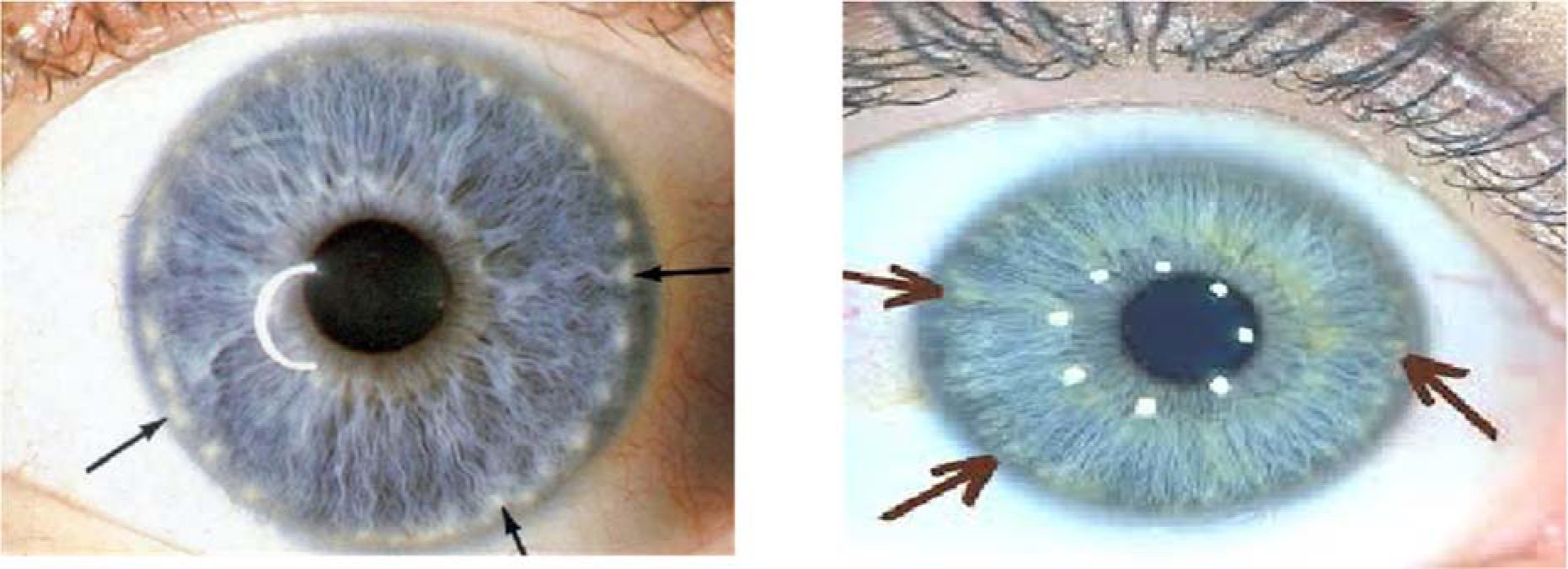
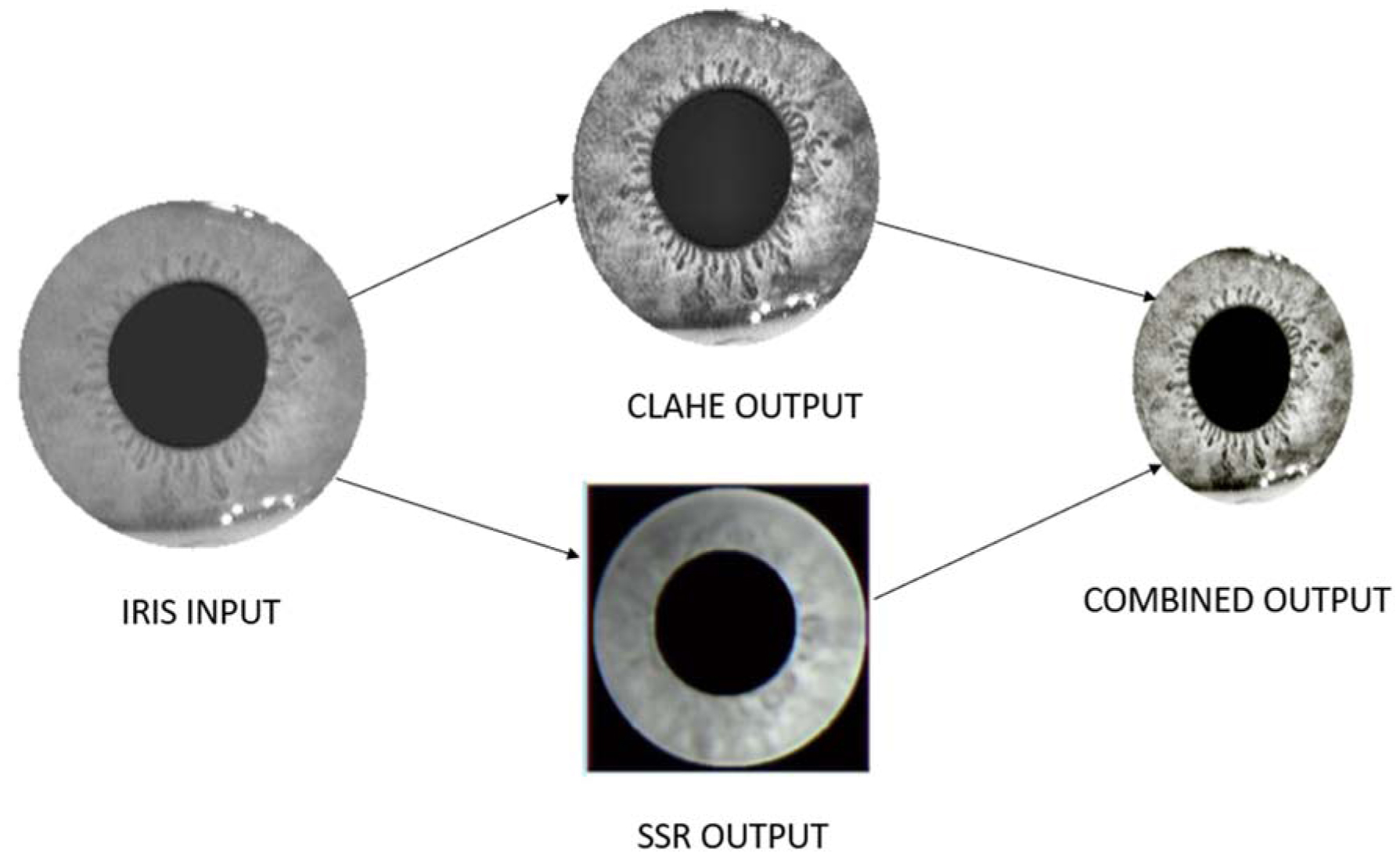
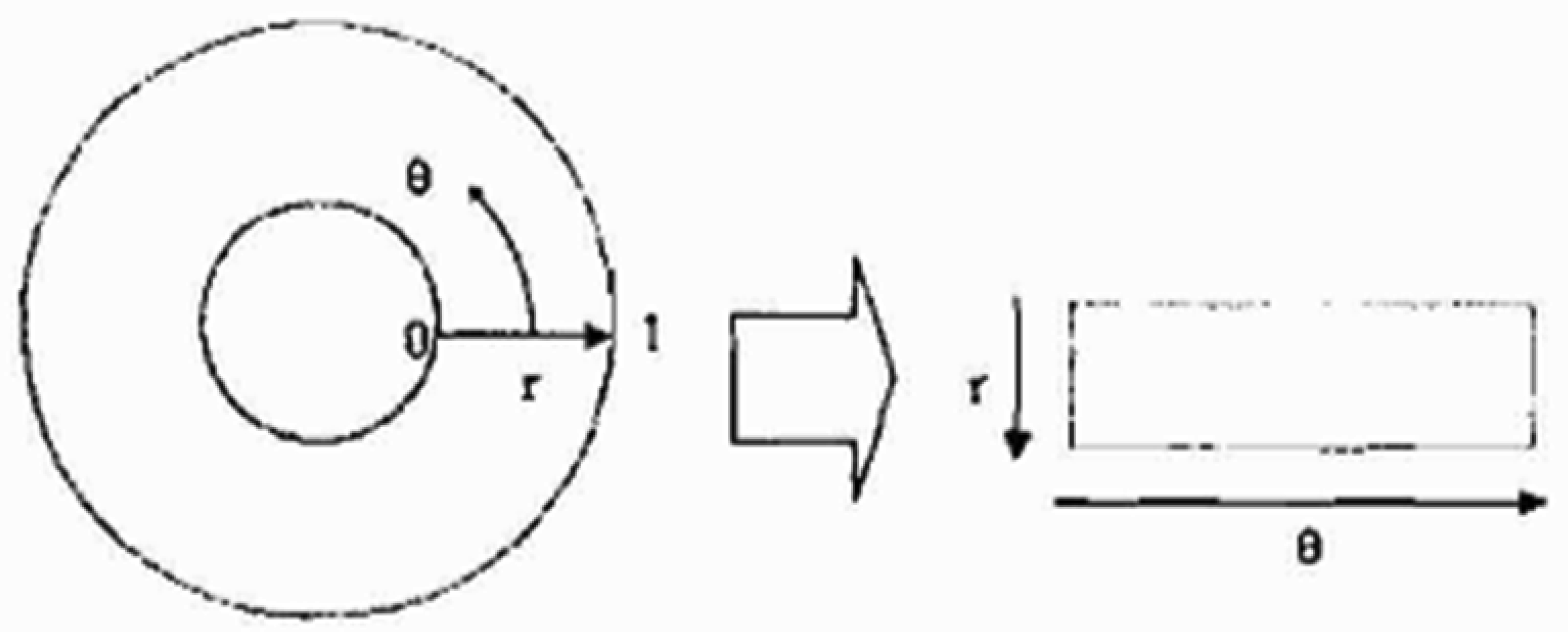
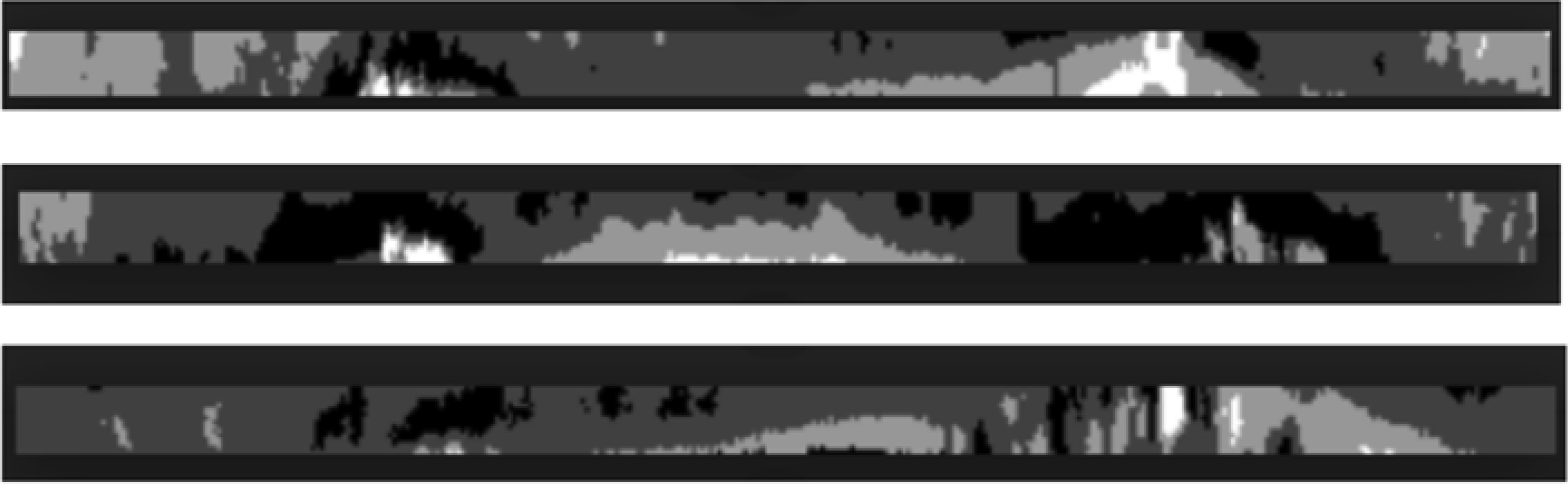
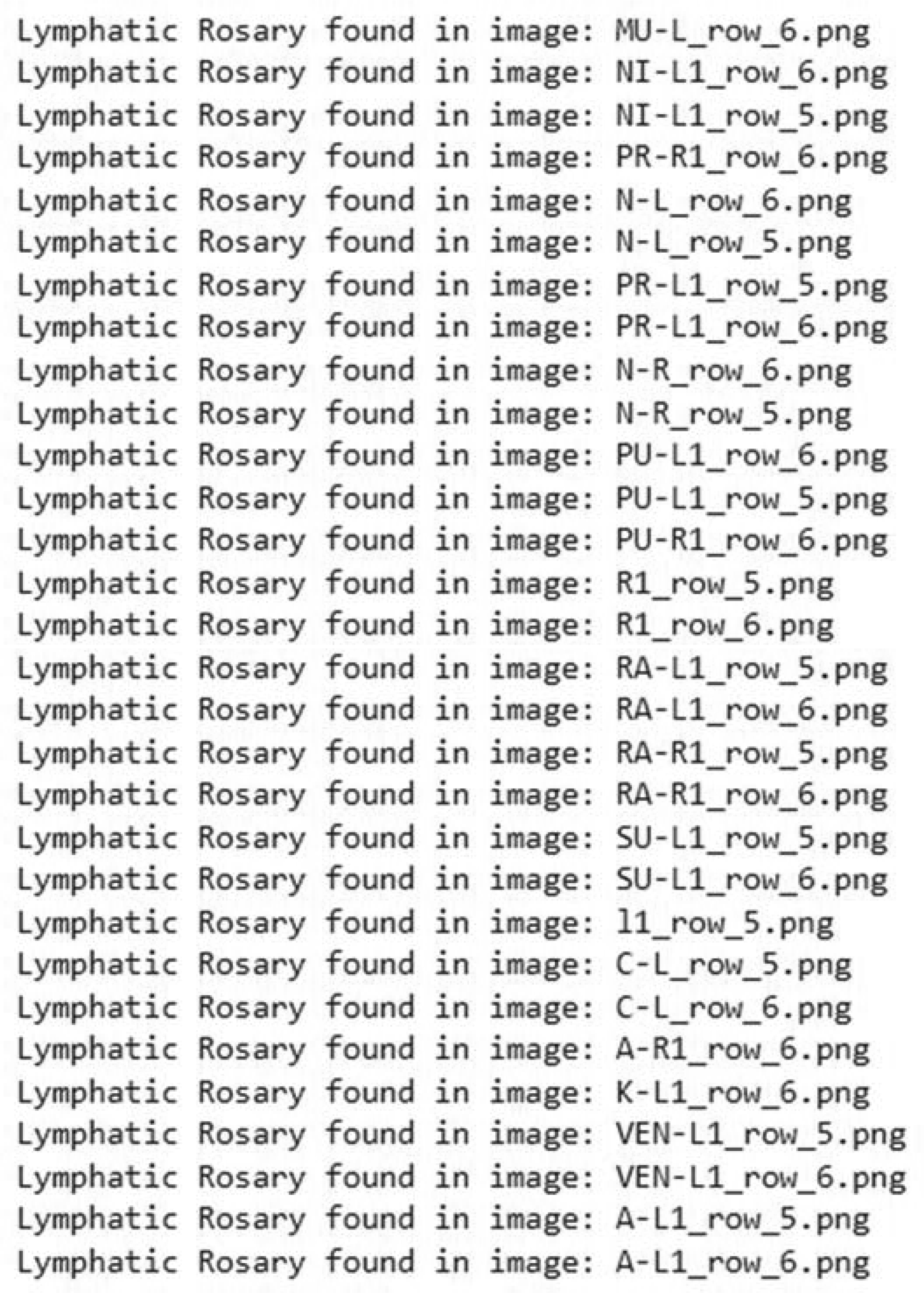
Lymphatic dysfunction is characterized by the sluggish movement of lymph fluids. It manifests as a “Lymphatic Rosary” in the iris which is often due to dehydration and inactivity. Detecting these signs early is crucial for diagnosis and treatment. Therefore, there is a need for an automated, accurate, and efficient method to detect lymphatic rosaries in the iris. This paper presents a novel approach for detecting a lymphatic rosary using advanced image processing techniques. The proposed method involves iris segmentation to isolate the iris from the eye, followed by normalization to standardize its structure, and concludes with the application of the modified Daugman method to identify the lymphatic rosary. This automated process aims to enhance the accuracy and reliability of detection by minimizing the subjectivity associated with manual analysis. The proposed approach was tested on various iris images and the results demonstrated impressive accuracy in detecting lymphatic rosaries. The use of different iris code bit representations allowed for a robust detection process, showcasing the method's effectiveness by achieving an accuracy of 94.5% in identifying the presence of a lymphatic rosary across different stages. The novel image processing technique outlined in this paper offers a promising solution for the automated detection of lymphatic rosaries in the iris. The approach not only improves diagnostic accuracy but also provides a standardized method that could be widely implemented in clinical settings. This advancement in iris diagnosis has the potential to play a significant role in the early detection and management of lymphatic dysfunction.

Keywords:

Citation: Poovayar Priya Mohan, Ezhilarasan Murugesan. A novel approach for detecting the presence of a lymphatic rosary in the iris using a 3-stage algorithm[J]. AIMS Bioengineering, 2024, 11(4): 506-526. doi: 10.3934/bioeng.2024023

Related Papers:

[1]	P. Pirmohabbati, A. H. Refahi Sheikhani, H. Saberi Najafi, A. Abdolahzadeh Ziabari . Numerical solution of full fractional Duffing equations with Cubic-Quintic-Heptic nonlinearities. AIMS Mathematics, 2020, 5(2): 1621-1641. doi: 10.3934/math.2020110
[2]	SAIRA, Wenxiu Ma, Suliman Khan . An efficient numerical method for highly oscillatory logarithmic-algebraic singular integrals. AIMS Mathematics, 2025, 10(3): 4899-4914. doi: 10.3934/math.2025224
[3]	Kai Wang, Guicang Zhang . Curve construction based on quartic Bernstein-like basis. AIMS Mathematics, 2020, 5(5): 5344-5363. doi: 10.3934/math.2020343
[4]	Taher S. Hassan, Amir Abdel Menaem, Hasan Nihal Zaidi, Khalid Alenzi, Bassant M. El-Matary . Improved Kneser-type oscillation criterion for half-linear dynamic equations on time scales. AIMS Mathematics, 2024, 9(10): 29425-29438. doi: 10.3934/math.20241426
[5]	Dexin Meng . Wronskian-type determinant solutions of the nonlocal derivative nonlinear Schrödinger equation. AIMS Mathematics, 2025, 10(2): 2652-2667. doi: 10.3934/math.2025124
[6]	Samia BiBi, Md Yushalify Misro, Muhammad Abbas . Smooth path planning via cubic GHT-Bézier spiral curves based on shortest distance, bending energy and curvature variation energy. AIMS Mathematics, 2021, 6(8): 8625-8641. doi: 10.3934/math.2021501
[7]	Chunli Li, Wenchang Chu . Remarkable series concerning $\binom{3n}{n}$ and harmonic numbers in numerators. AIMS Mathematics, 2024, 9(7): 17234-17258. doi: 10.3934/math.2024837
[8]	Beatriz Campos, Alicia Cordero, Juan R. Torregrosa, Pura Vindel . Dynamical analysis of an iterative method with memory on a family of third-degree polynomials. AIMS Mathematics, 2022, 7(4): 6445-6466. doi: 10.3934/math.2022359
[9]	A. Palanisamy, J. Alzabut, V. Muthulakshmi, S. S. Santra, K. Nonlaopon . Oscillation results for a fractional partial differential system with damping and forcing terms. AIMS Mathematics, 2023, 8(2): 4261-4279. doi: 10.3934/math.2023212
[10]	Tongzhu Li, Ruiyang Lin . Classification of Möbius homogeneous curves in $\mathbb{R}^4$ . AIMS Mathematics, 2024, 9(8): 23027-23046. doi: 10.3934/math.20241119

Abstract

1. Introduction

We consider the following family of nonlinear oscillators

$\begin{equation} y_{zz}+k(y)y_{z}^{3}+h(y)y_{z}^{2}+f(y)y_{z}+g(y) = 0, \end{equation}$

(1.1)

where $k$ , $h$ , $f\neq0$ and $g\neq0$ are arbitrary sufficiently smooth functions. Particular members of (1.1) are used for the description of various processes in physics, mechanics and so on and they also appear as invariant reductions of nonlinear partial differential equations ^[1,2,3].

Integrability of (1.1) was studied in a number of works ^{[4,5,6,7,8,9,10,11,12,13,14,15,16]}. In particular, in ^[15] linearization of (1.1) via the following generalized nonlocal transformations

$\begin{equation} w = F(y), \quad d\zeta = (G_{1}(y)y_{z}+G_{2}(y))dz. \end{equation}$

(1.2)

was considered. However, equivalence problems with respect to transformations (1.2) for (1.1) and its integrable nonlinear subcases have not been studied previously. Therefore, in this work we deal with the equivalence problem for (1.1) and its integrable subcase from the Painlevé-Gambier classification. Namely, we construct an equivalence criterion for (1.1) and a non-canonical form of Ince Ⅶ equation ^[17,18]. As a result, we obtain two new integrable subfamilies of (1.1). What is more, we demonstrate that for any equation from (1.1) that satisfy one of these equivalence criteria one can construct an autonomous first integral in the parametric form. Notice that we use Ince Ⅶ equation because it is one of the simplest integrable members of (1.1) with known general solution and known classification of invariant curves.

Moreover, we show that transformations (1.2) preserve autonomous invariant curves for equations from (1.1). Since the considered non-canonical form of Ince Ⅶ equation admits two irreducible polynomial invariant curves, we obtain that any equation from (1.1), which is equivalent to it, also admits two invariant curves. These invariant curves can be used for constructing an integrating factor for equations from (1.1) that are equivalent to Ince Ⅶ equation. If this integrating factor is Darboux one, then the corresponding equation is Liouvillian integrable ^[19]. This demonstrates the connection between nonlocal equivalence approach and Darboux integrability theory and its generalizations, which has been recently discussed for a less general class of nonlocal transformations in ^[20,21,22].

The rest of this work is organized as follows. In the next Section we present an equivalence criterion for (1.1) and a non-canonical form of the Ince Ⅶ equation. In addition, we show how to construct an autonomous first integral for an equation from (1.1) satisfying this equivalence criterion. We also demonstrate that transformations (1.2) preserve autonomous invariant curves for (1.1). In Section 3 we provide two examples of integrable equations from (1.1) and construct their parametric first integrals, invariant curves and integrating factors. In the last Section we briefly discuss and summarize our results.

2. Main results

We begin with the equivalence criterion between (1.1) and a non-canonical form of the Ince Ⅶ equation, that is ^[17,18]

$\begin{equation} w_{\zeta\zeta}+3w_{\zeta}+\epsilon w^{3}+2w = 0. \end{equation}$

(2.1)

Here $\epsilon\neq0$ is an arbitrary parameter, which can be set, without loss of generality, to be equal to $\pm 1$ .

The general solution of (1.1) is

$\begin{equation} w = {\rm e}^{-(\zeta-\zeta_{0})}\rm{cn}\left\{\sqrt{\epsilon}({\rm e}^{-(\zeta-\zeta_{0})}-C_{1}),\frac{1}{\sqrt{2}}\right\}. \end{equation}$

(2.2)

Here $\zeta_{0}$ and $C_{1}$ are arbitrary constants and $\rm{cn}$ is the Jacobian elliptic cosine. Expression (2.2) will be used below for constructing autonomous parametric first integrals for members of (1.1).

The equivalence criterion between (1.1) and (2.1) can be formulated as follows:

Theorem 2.1. Equation (1.1) is equivalent to (2.1) if and only if either

$\begin{equation} \begin{gathered} (I)\quad 25515lgp^{2}q_{y}+2352980l^{10}+\left(3430q-6667920p^{3}\right) l^{5}\\ -14580qp^{3}-10q^{2}-76545lgqpp_{y} = 0, \end{gathered} \end{equation}$

(2.3)

$\begin{equation} \begin{gathered} (II)\quad 343l^{5}-972p^{3} = 0, \end{gathered} \end{equation}$

(2.4)

holds. Here

$\begin{equation} \begin{gathered} l = 9(fg_{y}-gf_{y}+fgh-3kg^{2})-2f^{3}, \quad p = gl_{y}-3lg_{y}+l(f^{2}-3gh),\\ q = 25515g_{y}lp^{2}-5103lgpp_{y}+686l^{5}-8505p^{2}\left( f^{2}-3gh \right) l+6561p^{3}. \end{gathered} \end{equation}$

(2.5)

The expression for $G_{2}$ in each case is either

$\begin{equation} (I) \quad G_{2} = \frac {126 l^{2}qp^{2}}{470596 l^{10}- \left( 1333584 p^{3}+1372 q \right) l^{5}+q^{2}}, \end{equation}$

(2.6)

$\begin{equation} (II) \quad G_{2}^{2} = -\frac{49l^{3}G_{2}+9p^{2}}{189pl}. \end{equation}$

(2.7)

In all cases the functions $F$ and $G_{1}$ are given by

$\begin{equation} F^{2} = \frac{l}{81\epsilon G_{2}^{3}}, \quad G_{1} = \frac{G_{2}(f-3G_{2})}{3g}. \end{equation}$

(2.8)

Proof. We begin with the necessary conditions. Substituting (1.2) into (2.1) we get

$\begin{equation} y_{zz}+k(y)y_{z}^{3}+h(y)y_{z}^{2}+f(y)y_{z}+g(y) = 0, \end{equation}$

(2.9)

where

$\begin{equation} \begin{gathered} k = \frac{FG_{1}^{3}(\epsilon F^{2}+2)+3G_{1}^{2}F_{y}+G_{1}F_{yy}-F_{y}G_{1,y}}{G_{2}F_{y}}, \\ h = \frac{G_{2}F_{yy}+(6G_{1}G_{2}-G_{2,y})F_{y}+3FG_{2}G_{1}^{2}(\epsilon F^{2}+2)}{G_{2}F_{y}},\\ f = \frac{3G_{2}(F_{y}+FG_{1}(\epsilon F^{2}+2))}{F_{y}}, \quad g = \frac{FG_{2}^{2}(\epsilon F^{2}+2)}{F_{y}}. \end{gathered} \end{equation}$

(2.10)

As a consequence, we obtain that (1.1) can be transformed into (2.1) if it is of the form (2.9) (or (1.1)).

Conversely, if the functions $F$ , $G_{1}$ and $G_{2}$ satisfy (2.10) for some values of $k$ , $h$ , $f$ and $g$ , then (1.1) can be mapped into (2.1) via (1.2). Thus, we see that the compatibility conditions for (2.10) as an overdertmined system of equations for $F$ , $G_{1}$ and $G_{2}$ result in the necessary and sufficient conditions for (1.1) to be equivalent to (2.1) via (1.2).

To obtain the compatibility conditions, we simplify system (2.10) as follows. Using the last two equations from (2.10) we find the expression for $G_{1}$ given in (2.8). Then, with the help of this relation, from (2.10) we find that

$\begin{equation} 81\epsilon F^{2}G_{2}^{3}-l = 0, \end{equation}$

(2.11)

and

$\begin{equation} \begin{gathered} 567lG_{2}^{3}+(243lgh-81lf^{2}-81gl_{y}+243lg_{y})G_{2}-7l^{2} = 0,\\ 243lgG_{2,y}+324lG_{2}^{3}-81gl_{y}G_{2}+2l^{2} = 0, \end{gathered} \end{equation}$

(2.12)

Here $l$ is given by (2.5).

As a result, we need to find compatibility conditions only for (2.12). In order to find the generic case of this compatibility conditions, we differentiate the first equation twice and find the expression for $G_{2}^{2}$ and condition (2.3). Differentiating the first equation from (2.12) for the third time, we obtain (2.6). Further differentiation does not lead to any new compatibility conditions. Particular case (2.4) can be treated in the similar way.

Finally, we remark that the cases of $l = 0$ , $p = 0$ and $q = 0$ result in the degeneration of transformations (1.2). This completes the proof.

As an immediate corollary of Theorem 2.1 we get

Corollary 2.1. If coefficients of an equation from (1.1) satisfy either (2.3) or (2.4), then an autonomous first integral of this equation can be presented in the parametric form as follows:

$\begin{equation} y = F^{-1}(w), \quad y_{z} = \frac{G_{2}w_{\zeta}}{F_{y}-G_{1}w_{\zeta}}\,. \end{equation}$

(2.13)

Here $w$ is the general solution of (2.1) given by (2.2). Notice also that, formally, (2.13) contains two arbitrary constants, namely $\zeta_{0}$ and $C_{1}$ . However, without loss of generality, one of them can be set equal to zero.

Now we demonstrate that transformations (1.2) preserve autonomous invariant curves for equations from (1.1).

First, we need to introduce the definition of an invariant curve for (1.1). We recall that Eq (1.1) can be transformed into an equivalent dynamical system

$\begin{equation} y_{z} = P, \quad u_{z} = Q, \quad P = u, \quad Q = -k u^{3}-h u^{2}-f u -g. \end{equation}$

(2.14)

A smooth function $H(y, u)$ is called an invariant curve of (2.14) (or, equivalently, of (1.1)), if it is a nontrivial solution of ^[19]

$\begin{equation} PH_{y}+QH_{u} = \lambda H, \end{equation}$

(2.15)

for some value of the function $\lambda$ , which is called the cofactor of $H$ .

Second, we need to introduce the equation that is equivalent to (1.1) via (1.2). Substituting (1.2) into (1.1) we get

$\begin{equation} w_{\zeta\zeta}+\tilde{k}w_{\zeta}^{3}+\tilde{h}w_{\zeta}^{2}+\tilde{f}w_{\zeta}+\tilde{g} = 0, \end{equation}$

(2.16)

where

$\begin{equation} \begin{gathered} \tilde{k} = \frac{kG_{2}^{3}-gG_{1}^{3}+(G_{1,y}-hG_{1})G_{2}^{2}+(fG_{1}-G_{2,y})G_{1}G_{2}}{F_{y}^{2}G_{2}^{2}},\\ \tilde{h} = \frac{(hF_{y}-F_{yy})G_{2}^{2}-(2fG_{1}-G_{2,y})G_{2}F_{y}+3gG_{1}^{2}F_{y}}{F_{y}^{2}G_{2}^{2}},\\ \tilde{f} = \frac{fG_{2}-3gG_{1}}{G_{2}^{2}}, \quad \tilde{g} = \frac{gF_{y}}{G_{2}^{2}}. \end{gathered} \end{equation}$

(2.17)

An invariant curve for (2.16) can be defined in the same way as that for (1.1). Notice that, further, we will denote $w_{\zeta}$ as $v$ .

Theorem 2.2. Suppose that either (1.1) possess an invariant curve $H(y, u)$ with the cofactor $\lambda(y, u)$ or (2.16) possess an invariant curve $\widetilde{H}(w, v)$ with the cofactor $\tilde{\lambda}(w, v)$ . Then, the other equation also has an invariant curve and the corresponding invariant curves and cofactors are connected via

$\begin{equation} \begin{gathered} H(y,u) = \widetilde{H}\left(F,\frac{F_{y}u}{G_{1}u+G_{2}}\right), \quad \lambda(y,u) = (G_{1}u+G_{2})\tilde{\lambda}\left(F,\frac{F_{y}u}{G_{1}u+G_{2}}\right). \end{gathered} \end{equation}$

(2.18)

Proof. Suppose that $\widetilde{H}(w, v)$ is an invariant curve for (2.16) with the cofactor $\widetilde{\lambda}(w, v)$ . Then it satisfies

$\begin{equation} v\widetilde{H}_{w}+(-\tilde{k} v^{3}-\tilde{h} v^{2}-\tilde{f} v -\tilde{g})\widetilde{H}_{v} = \widetilde{\lambda}\widetilde{H}. \end{equation}$

(2.19)

Substituting (1.2) into (2.19) we get

$\begin{equation} uH_{y}+(-k u^{3}-h u^{2}-f u-g)H = (G_{1}u+G_{2}) \tilde{\lambda}\left(F,\frac{F_{y}u}{G_{1}u+G_{2}}\right) H . \end{equation}$

(2.20)

This completes the proof.

As an immediate consequence of Theorem 2.2 we have that transformations (1.2) preserve autonomous first integrals admitted by members of (1.1), since they are invariant curves with zero cofactors.

Another corollary of Theorem 2.2 is that any equation from (1.1) that is connected to (2.1) admits two invariant curves that correspond to irreducible polynomial invariant curves of (2.1). This invariant curves of (2.1) and the corresponding cofactors are the following (see, ^[23] formulas (3.18) and (3.19) taking into account scaling transformations)

$\begin{equation} \widetilde{H} = \pm i \sqrt{-2\epsilon}(v+w)+w^{2}, \quad \tilde{\lambda} = \pm \sqrt{-2\epsilon}w-2. \end{equation}$

(2.21)

Therefore, we have that the following statement holds:

Corollary 2.2. If coefficients of an equation from (1.1) satisfy either (2.3) or (2.4), then is admits the following invariant curves with the corresponding cofactors

$\begin{equation} H = \pm i \sqrt{-2\epsilon}\left(\frac{F_{y}u}{G_{1}u+G_{2}}+F\right)+F^{2}, \quad \lambda = \left(G_{1}u+G_{2}\right)\left(\pm \sqrt{-2\epsilon}F-2\right). \end{equation}$

(2.22)

Let us remark that connections between (2.1) and non-autonomous variants of (1.1) can be considered via a non-autonomous generalization of transformations (1.2). However, one of two nonlocally related equations should be autonomous since otherwise nonlocal transformations do not map a differential equation into a differential equation ^[5].

In this Section we have obtained the equivalence criterion between (1.1) and (2.1), that defines two new completely integrable subfamilies of (1.1). We have also demonstrated that members of these subfamilies posses an autonomous parametric first integral and two autonomous invariant curves.

3. Examples

In this Section we provide two examples of integrable equations from (1.1) satisfying integrability conditions from Theorem 2.1.

Example 1. One can show that the coefficients of the following cubic oscillator

$\begin{equation} y_{zz}-\frac{12\epsilon \mu y}{(\epsilon \mu^{2}y^{4}+2)^{2}}y_{z}^{3}-6\mu y y_{z}+2\mu^{2}y^{3}(\epsilon\mu^{2}y^{4}+2) = 0, \end{equation}$

(3.1)

satisfy condition (2.3) from Theorem 2.1. Consequently, Eq (3.1) is completely integrable and its general solution can be obtained from (2.2) by inverting transformations (1.2). However, it is more convenient to use Corollary 2.1 and present the autonomous first integral of (3.1) in the parametric form as follows:

$\begin{equation} y = \pm\sqrt{\frac{w}{\mu}}, \quad y_{z} = \frac{w(\epsilon w^{2}+2) w_{\zeta}}{2w_{\zeta}+w(\epsilon w^{2}+2)}, \end{equation}$

(3.2)

where $w$ is given by (2.2), $\zeta$ is considered as a parameter and $\zeta_{0}$ , without loss of generality, can be set equal to zero. As a result, we see that (3.1) is integrable since it has an autonomous first integral.

Moreover, using Corollary 2.2 one can find invariant curves admitted by (3.1)

$\begin{equation} \begin{gathered} H_{1,2} = \frac{y^{4}\left[(\sqrt{2}\pm \sqrt{-\epsilon}\mu y^{2})^{2}(\sqrt{2}\mp\sqrt{-\epsilon}\mu y^{2})+2(\epsilon\mu y^{2}\mp\sqrt{-2\epsilon})u\right]}{2\mu^{2}y^{2}(\epsilon\mu^{2}y^{4}+2)-4u},\\ \lambda_{1,2} = \pm\frac{2(\mu y^{2}(\epsilon\mu^{2}y^{4}+2)-2u)(\sqrt{-2\epsilon}\mu y^{2}\mp 2)}{y(\epsilon\mu^{2}y^{4}+2)} \end{gathered} \end{equation}$

(3.3)

With the help of the standard technique of the Darboux integrability theory ^[19], it is easy to find the corresponding Darboux integrating factor of (3.1)

$\begin{equation} M = \frac{(\epsilon \mu^{2}y^{4}+2)^{\frac{9}{4}}}{(2\epsilon u^{2}+(\epsilon\mu^{2}y^{4}+2)^{2})^{\frac{3}{4}}(\mu y^{2}(\epsilon \mu^{2}y^{4}+2)-2u)^{\frac{3}{2}}}. \end{equation}$

(3.4)

Consequently, equation is (3.1) Liouvillian integrable.

Example 2. Consider the Liénard (1, 9) equation

$\begin{equation} y_{zz}+(b_{i}y^{i}){y_{z}}+a_{j}y^{j} = 0, \quad i = 0,\ldots 4, \quad j = 0,\ldots,9. \end{equation}$

(3.5)

Here summation over repeated indices is assumed. One can show that this equation is equivalent to (2.1) if it is of the form

$\begin{equation} y_{zz}-9(y+\mu)(y+3\mu)^{3}y_{z}+2y(2y+3\mu)(y+3\mu)^{7} = 0, \end{equation}$

(3.6)

where $\mu$ is an arbitrary constant.

With the help of Corollary 2.1 one can present the first integral of (3.6) in the parametric form as follows:

$\begin{equation} y = \frac{3\sqrt{-2\epsilon}\mu w}{2-\sqrt{-2\epsilon}w}, \quad y_{z} = \frac{7776 \sqrt{2} \epsilon \mu^{5} w w_{\zeta}}{(\sqrt{-2\epsilon}w-2)^{5}(2\sqrt{-\epsilon}w_{\zeta}+(\sqrt{2}\epsilon w +2\sqrt{-\epsilon})w)}, \end{equation}$

(3.7)

where $w$ is given by (2.2). Thus, one can see that (3.5) is completely integrable due to the existence of this parametric autonomous first integral.

Using Corollary 2.2 we find two invariant curves of (3.6):

$\begin{equation} H_{1} = \frac{y^{2}[(2y+3\mu)(y+3\mu)^{4}-2u)]}{(y+3\mu)^{2}[(y+3\mu)^{4}y-u]}, \quad \lambda_{1} = \frac{6\mu(u-y(y+3\mu)^{4})}{y(y+3\mu)}, \end{equation}$

(3.8)

and

$\begin{equation} H_{2} = \frac{y^{2}(y+3\mu)^{2}}{y(y+3\mu)^{4}-u}, \quad \lambda_{2} = \frac{2(2y+3\mu)(u-2y(y+3\mu)^{4})}{y(y+3\mu)}. \end{equation}$

(3.9)

The corresponding Darboux integrating factor is

$\begin{equation} M = \left[y(y+3\mu)^{4}-u\right]^{-\frac{3}{2}}\left[(2y+3\mu)(y+3\mu)^{4}-2u\right]^{-\frac{3}{4}}. \end{equation}$

(3.10)

As a consequence, we see that Eq (3.6) is Liouvillian integrable.

Therefore, we see that equations considered in Examples 1 and 2 are completely integrable from two points of view. First, they possess autonomous parametric first integrals. Second, they have Darboux integrating factors.

4. Conclusions and discussion

In this work we have considered the equivalence problem between family of Eqs (1.1) and its integrable member (2.1), with equivalence transformations given by generalized nonlocal transformations (1.2). We construct the corresponding equivalence criterion in the explicit form, which leads to two new integrable subfamilies of (1.1). We have demonstrated that one can explicitly construct a parametric autonomous first integral for each equation that is equivalent to (2.1) via (1.2). We have also shown that transformations (1.2) preserve autonomous invariant curves for (1.1). As a consequence, we have obtained that equations from the obtained integrable subfamilies posses two autonomous invariant curves, which corresponds to the irreducible polynomial invariant curves of (2.1). This fact demonstrate a connection between nonlocal equivalence approach and Darboux and Liouvillian integrability approach. We have illustrate our results by two examples of integrable equations from (1.1).

Acknowledgments

The author was partially supported by Russian Science Foundation grant 19-71-10003.

Conflict of interest

The author declares no conflict of interest in this paper.

Conflict of interest

The authors declare that they have no known competing financial interests or personal relationships that could have influenced the work reported in this paper.

Author contributions

Poovayar Priya M. provided the conceptualization, investigation, methodology, implementation, validation, and visualization, and wrote the original draft; Ezhilarasan M. provided the validation and supervision.

References

[1]	Sharan F (1989) Iridology: A Complete Guide to Diagnosing through the Iris and to Related Forms of Treatment. New York: HarperThorsons.
[2]	Jensen B (1980) Iridology Simplified. Canada: Book Publishing Company.
[3]	Kryzhanivska O (2020) Iris changes at patients with temporomandibular joint diseases and urinary system pathology. MSU 16: 28-34. https://doi.org/10.32345/2664-4738.4.2020.5
[4]	Sen M, Honavar SG (2022) Theodor karl gustav von leber: the sultan of selten. Indian J Ophthalmol 70: 2218-2220. https://doi.org/10.4103/ijo.IJO_1379_22
[5]	de Oliveira ER, de Souza Cardoso J, da Silva Rodrigues VT, et al. (2023) Nocardia niwae infection in dogs. Acta Sci Vet 51: 900. https://doi.org/10.22456/1679-9216.131057
[6]	Caruso M, Catalano O, Bard R, et al. (2022) Non-glandular findings on breast ultrasound. Part I: a pictorial review of superficial lesions. J ultrasound 25: 783-797. https://doi.org/10.1007/s40477-021-00619-2
[7]	Jogi SP, Sharma BB Retracted: methodology of iris image analysis for clinical diagnosis. (2014)2014: 235-240. https://doi.org/10.1109/MedCom.2014.7006010
[8]	Atkin S (2013) Bilateral pitting oedema with multiple aetiologies. Aust J Herbal Med 25: 79-82. https://doi.org/10.3316/informit.481869825723186
[9]	Jensen B (1982) Iridology: Science and Practice in the Healing Arts. Canada: Book Publishing Company.
[10]	Gu R, Wang G, Song T, et al. (2020) CA-Net: comprehensive attention convolutional neural networks for explainable medical image segmentation. IEEE T Med Imaging 40: 699-711. https://doi.org/10.1109/TMI.2020.3035253
[11]	Touvron H, Cord M, Douze M, et al. Training data-efficient image transformers & distillation through attention. (2021)139: 10347-10357.
[12]	Wang Y, Seo J, Jeon T (2021) NL-LinkNet: toward lighter but more accurate road extraction with nonlocal operations. IEEE Geosci Remote S 19: 1-5. https://doi.org/10.1109/LGRS.2021.3050477
[13]	Chen Z, Zeng H, Yang W, et al. Texture enhancement method of oceanic internal waves in SAR images based on non-local mean filtering and multi-scale retinex. (2022)2022: 1-5. https://doi.org/10.1109/CISS57580.2022.9971169
[14]	Agrawal S, Panda R, Mishro PK, et al. (2022) A novel joint histogram equalization-based image contrast enhancement. J King Saud Univ-Com 34: 1172-1182. https://doi.org/10.1016/j.jksuci.2019.05.010
[15]	Rao BS (2020) Dynamic histogram equalization for contrast enhancement for digital images. Appl Soft Comput 89: 106114. https://doi.org/10.1016/j.asoc.2020.106114
[16]	Doshvarpassand S, Wang X, Zhao X (2022) Sub-surface metal loss defect detection using cold thermography and dynamic reference reconstruction (DRR). Struct Health Monit 21: 354-369. https://doi.org/10.1177/1475921721999599
[17]	Murugachandravel J, Anand S (2021) Enhancing MRI brain images using contourlet transform and adaptive histogram equalization. J Med Imag Health In 11: 3024-3027. https://doi.org/10.1166/jmihi.2021.3906
[18]	Radzi SFM, Karim MKA, Saripan MI, et al. (2020) Impact of image contrast enhancement on the stability of radiomics feature quantification on a 2D mammogram radiograph. IEEE Access 8: 127720-127731. https://doi.org/10.1109/ACCESS.2020.3008927
[19]	Kuran U, Kuran EC (2021) Parameter selection for CLAHE using multi-objective cuckoo search algorithm for image contrast enhancement. Intell Syst Appl 12: 200051. https://doi.org/10.1016/j.iswa.2021.200051
[20]	Islam MR, Nahiduzzaman M (2022) Complex features extraction with deep learning model for the detection of COVID-19 from CT scan images using ensemble-based machine learning approach. Expert Syst Appl 195: 116554. https://doi.org/10.1016/j.eswa.2022.116554
[21]	Chen Y, Xia R, Yang K, et al. (2024) MICU: image super-resolution via multi-level information compensation and U-net. Expert Syst Appl 245: 123111. https://doi.org/10.1016/j.eswa.2023.123111
[22]	Chen Y, Xia R, Yang K, et al. (2024) DNNAM: image inpainting algorithm via deep neural networks and attention mechanism. Appl Soft Comput 154: 111392. https://doi.org/10.1016/j.asoc.2024.111392
[23]	Chen Y, Xia R, Yang K, et al. (2024) MFMAM: image inpainting via multi-scale feature module with attention module. Comput Vis Image Und 238: 103883. https://doi.org/10.1016/j.cviu.2023.103883
[24]	Naeem AB, Senapati B, Bhuva D, et al. (2024) Heart disease detection using feature extraction and artificial neural networks: a sensor-based approach. IEEE Access 12: 37349-37362. https://doi.org/10.1109/ACCESS.2024.3373646
[25]	Mira ES, Sapri AMS, Aljehanı RF, et al. (2024) Early diagnosis of oral cancer using image processing and artificial intelligence. Fusion: Pract Appl 14: 293-308. https://doi.org/10.54216/FPA.140122
[26]	Kumar K, Pradeepa M, Mahdal M, et al. (2023) A deep learning approach for kidney disease recognition and prediction through image processing. Appl Sci 13: 3621. https://doi.org/10.3390/app13063621
[27]	Priyal MP, Ezhilarasan M IRIS segmentation technique using IRIS-UNet method. (2023)14124: 235. https://doi.org/10.1007/978-3-031-45382-3_20
[28]	Yang Y, Jiang Z, Yang C, et al. Improved retinex image enhancement algorithm based on bilateral filtering. (2015)2015: 1363-1369. https://doi.org/10.2991/icmmcce-15.2015.427
[29]	Daugman J (2007) New methods in iris recognition. IEEE T Syst Man Cy B 37: 1167-1175. https://doi.org/10.1109/TSMCB.2007.903540

This article has been cited by:

1.	Dmitry I. Sinelshchikov, Linearizabiliy and Lax representations for cubic autonomous and non-autonomous nonlinear oscillators, 2023, 01672789, 133721, 10.1016/j.physd.2023.133721
2.	Jaume Giné, Xavier Santallusia, Integrability via algebraic changes of variables, 2024, 184, 09600779, 115026, 10.1016/j.chaos.2024.115026
3.	Meryem Belattar, Rachid Cheurfa, Ahmed Bendjeddou, Paulo Santana, A class of nonlinear oscillators with non-autonomous first integrals and algebraic limit cycles, 2023, 14173875, 1, 10.14232/ejqtde.2023.1.50
4.	Jaume Giné, Dmitry Sinelshchikov, Integrability of Oscillators and Transcendental Invariant Curves, 2025, 24, 1575-5460, 10.1007/s12346-024-01182-x

Reader Comments

Your name:*

Email:*
© 2024 the Author(s), licensee AIMS Press. This is an open access article distributed under the terms of the Creative Commons Attribution License (http://creativecommons.org/licenses/by/4.0)