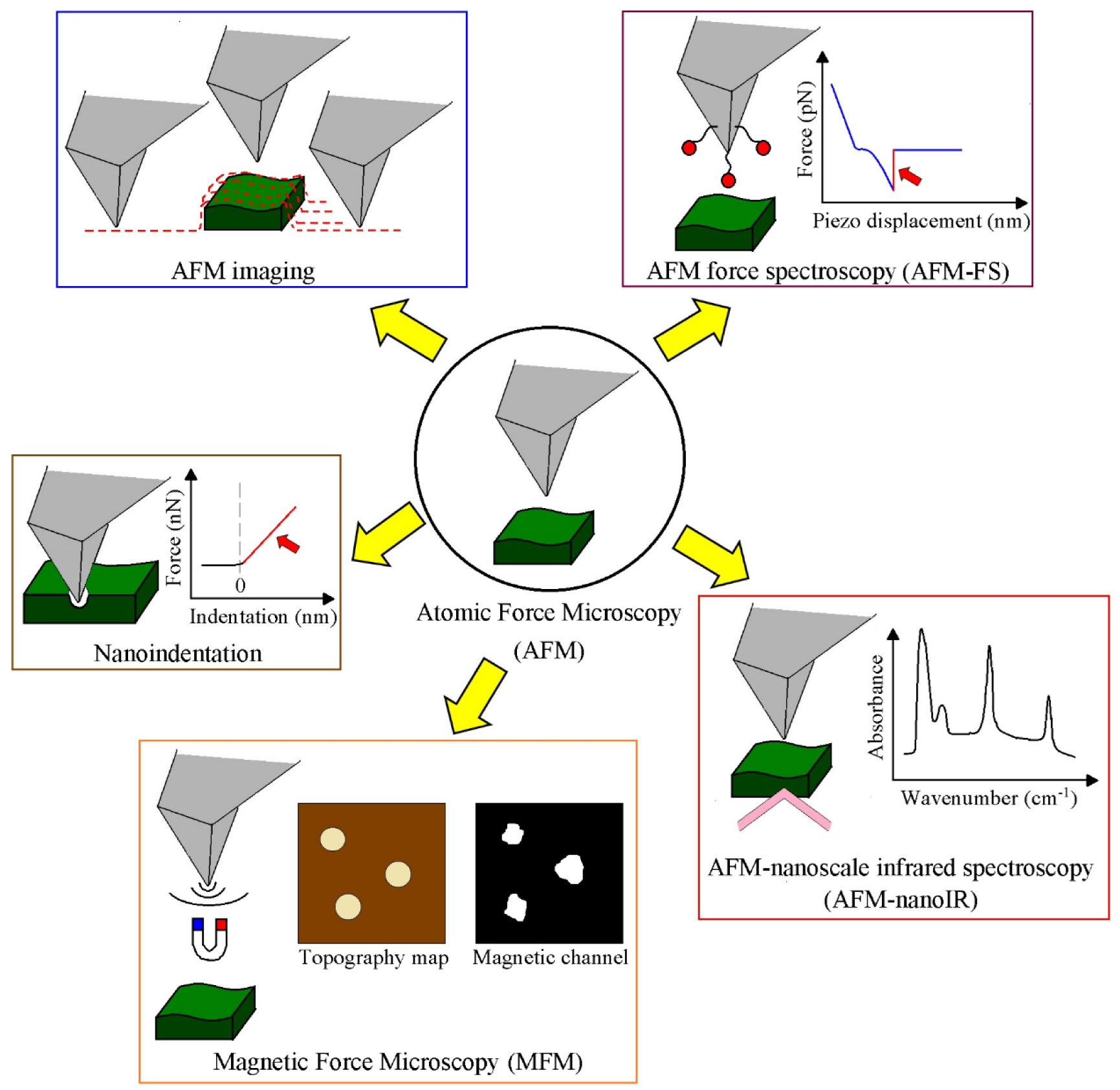
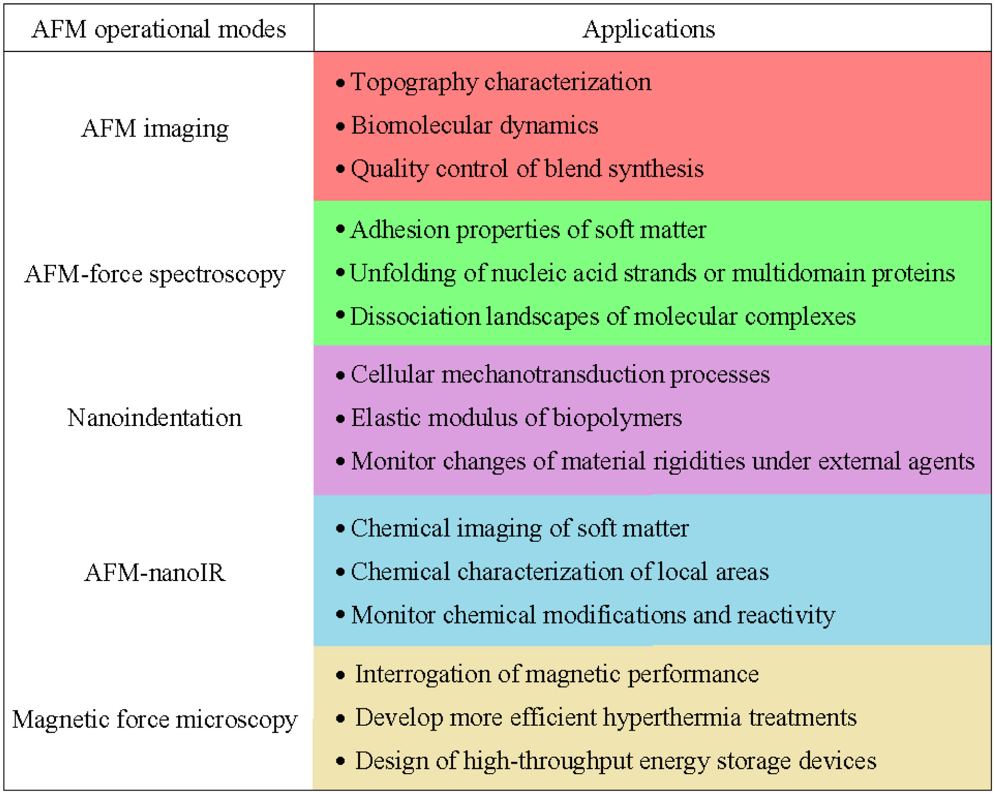
Soft matter encompasses multitude of systems like biomolecules, living cells, polymers, composites or blends. The increasing interest to better understand their physico-chemical properties has significantly favored the development of new techniques with unprecedented resolution. In this framework, atomic force microscopy (AFM) can act as one main actor to address multitude of intrinsic sample characteristics at the nanoscale level. AFM presents many advantages in comparison to other bulk techniques as the assessment of individual entities discharging thus, ensemble averaging phenomena. Moreover, AFM enables the visualization of singular events that eventually can provide response of some open questions that still remain unclear. The present manuscript aims to make the reader aware of the potential applications in the employment of this tool by providing recent examples of scientific studies where AFM has been employed with success. Several operational modes like AFM imaging, AFM based force spectroscopy (AFM-FS), nanoindentation, AFM-nanoscale infrared spectroscopy (AFM-nanoIR) or magnetic force microscopy (MFM) will be fully explained to detail the type of information that AFM is capable to gather. Finally, future prospects will be delivered to discern the following steps to be conducted in this field.
Citation: Carlos Marcuello. Current and future perspectives of atomic force microscopy to elicit the intrinsic properties of soft matter at the single molecule level[J]. AIMS Bioengineering, 2022, 9(3): 293-306. doi: 10.3934/bioeng.2022020
Soft matter encompasses multitude of systems like biomolecules, living cells, polymers, composites or blends. The increasing interest to better understand their physico-chemical properties has significantly favored the development of new techniques with unprecedented resolution. In this framework, atomic force microscopy (AFM) can act as one main actor to address multitude of intrinsic sample characteristics at the nanoscale level. AFM presents many advantages in comparison to other bulk techniques as the assessment of individual entities discharging thus, ensemble averaging phenomena. Moreover, AFM enables the visualization of singular events that eventually can provide response of some open questions that still remain unclear. The present manuscript aims to make the reader aware of the potential applications in the employment of this tool by providing recent examples of scientific studies where AFM has been employed with success. Several operational modes like AFM imaging, AFM based force spectroscopy (AFM-FS), nanoindentation, AFM-nanoscale infrared spectroscopy (AFM-nanoIR) or magnetic force microscopy (MFM) will be fully explained to detail the type of information that AFM is capable to gather. Finally, future prospects will be delivered to discern the following steps to be conducted in this field.

| [1] |
Binnig G, Quate CF, Gerber C (1986) Atomic force microcopy. Phys Rev Lett 56: 930-933. https://doi.org/10.1103/PhysRevLett.56.930 
|
| [2] |
Liu H, Li Y, Zhang Y, et al. (2018) Intelligent tuning method of PID parameters based on iterative learning control for atomic force microscopy. Micron 104: 26-36. https://doi.org/10.1016/j.micron.2017.09.009
|
| [3] |
Valotteau C, Sumbul F, Rico F (2019) High-speed force spectroscopy: microsecond force measurements using ultrashort cantilevers. Biophys Rev 11: 689-699. https://doi.org/10.1007/s12551-019-00585-4
|
| [4] |
Ando T (2018) High-speed atomic force microscopy and its future prospects. Biophys Rev 10: 285-292. https://doi.org/10.1007/s12551-017-0356-5
|
| [5] |
Marcuello C, Arilla-Luna S, Medina M, et al. (2013) Detection of a quaternary organization into dimer of trimers of Corynebacterium ammoniagenes FAD synthetase at the single-molecule level and at the in cell level. Biochim Biophys Acta 1834: 665-676. https://doi.org/10.1016/j.bbapap.2012.12.013
|
| [6] |
Vega S, Neira JL, Marcuello C, et al. (2013) NS3 protease from hepatitis C virus:biophysical studies on an intrinsically disordered protein domain. Int J Mol Sci 14: 13282-13306. https://doi.org/10.3390/ijms140713282
|
| [7] |
Villanueva R, Ferreira P, Marcuello C, et al. (2015) Key residues regulation the reductase activity of the human mitochondrial apoptosis inducing factor. Biochemistry 54: 5175-5184. https://doi.org/10.1021/acs.biochem.5b00696
|
| [8] |
Sebastián M, Lira-Navarrete E, Serrano A, et al. (2017) The FAD synthetase from the human pathogen Streptococcus penumoniae: a bifunctional enzyme exhibiting activity-dependent redox requirements. Sci Rep 7: 7609. https://doi.org/10.1038/s41598-017-07716-5
|
| [9] |
Song Q, Mao Y, Wilkins M, et al. (2016) Cellulase immobilization on superparamagnetic nanoparticles for reuse in cellulosic biomass conversion. AIMS Bioeng 3: 264-276. https://doi.org/10.3934/bioeng.2016.3.264
|
| [10] |
Ceballos-Laita L, Marcuello C, Lostao A, et al. (2017) Microcystin-LR binds Iron, and Iron promotes self-assembly. Environ Sci Technol 51: 4841-4850. https://doi.org/10.1021/acs.est.6b05939
|
| [11] |
Gerbin E, Frapart Y-M, Marcuello C, et al. (2020) Dual antioxidant properties and organic radical stabilization in cellulose nanocomposite films functionalized by in situ polymerization of coniferyl alcohol. Biomacromolecules 21: 3163-3175. https://doi.org/10.1021/acs.biomac.0c00583
|
| [12] |
Gerbin E, Rivière GN, Foulon L, et al. (2021) Tuning the functional properties of lignocellulosic films by controlling the molecular and supramolecular structure of lignin. Int J Biol Macromol 181: 136-149. https://doi.org/10.1016/j.ijbiomac.2021.03.081
|
| [13] |
Leung C, Kinns H, Hoogenboom BW, et al. (2009) Imaging surface charges of individual biomolecules. Nano Lett 9: 2769-2773. https://doi.org/10.1021/nl9012979
|
| [14] |
Seelert H, Poetsch A, Dencher NA, et al. (2000) Structural biology. Proton-powered turbine of a plant motor. Nature 405: 418-419. https://doi.org/10.1038/35013148
|
| [15] |
Fotiadis D, Liang Y, Filipek S, et al. (2003) Atomic-force microscopy: Rhodopsin dimers in native disc membranes. Nature 421: 127-128. https://doi.org/10.1038/421127a
|
| [16] |
Wong OK, Guthold M, Erie DA, et al. (2008) Interconvertible lac repressor-DNA loops revealed by single-molecule experiments. PLoS Biol 6: e232. https://doi.org/10.1371/journal.pbio.0060232
|
| [17] |
Pallarés MC, Marcuello C, Botello-Morte L, et al. (2014) Sequential binding of FurA from Anabaena sp. PCC 7120 to iron boxes: exploring regulation at the nanoscale. Biochim Biophys Acta 1844: 623-631. https://doi.org/10.1016/j.bbapap.2014.01.005
|
| [18] |
Nakata E, Dinh H, Nguyen TM, et al. (2019) DNA binding adaptors to assemble proteins of interest on DNA scaffold. Methods Enzymol 617: 287-322. https://doi.org/10.1016/bs.mie.2018.12.014
|
| [19] |
Müller DJ, Dufrêne YF (2008) Atomic force microscopy as a multifunctional molecular toolbox in nanobiotechnology. Nat Nanotechnol 3: 261-269. https://doi.org/10.1038/nnano.2008.100
|
| [20] |
Allison DP, Hinterdorfer P, Han W (2002) Biomolecular force measurements and the atomic force microscope. Curr Opin Biotechnol 13: 47-51. https://doi.org/10.1016/s0958-1669(02)00283-5
|
| [21] |
Müller DJ, Krieg M, Alsteen D, et al. (2009) New frontiers in atomic force microscopy: analyzing interactions from single-molecules to cells. Curr Opin Biotechnol 20: 4-13. https://doi.org/10.1016/j.copbio.2009.02.005
|
| [22] |
Rief M, Gautel M, Oesterhelt F, et al. (1997) Science276: 1109-1112. https://doi.org/10.1126/science.273.5315.1109
|
| [23] |
Giganti D, Yan K, Badilla CL, et al. (2018) Disulfide isomerization reactions in titin immunoglobulin domains enable a mode of protein elasticity. Nat Commun 9: 185. https://doi.org/10.1038/s41467-017-02528-7
|
| [24] |
Lipiec E, Sofinska K, Seweryn S, et al. (2021) Revealing DNA Structure at Liquid/Solid Interfaces by AFM-Based High-Resolution Imaging and Molecular Spectroscopy. Molecules 26: 6476. https://doi.org/10.3390/molecules26216476
|
| [25] |
Liu Y, Tian F, Shi S, et al. (2021) Enzymatic Protein-Protein Conjugation through Internal Site Verified at the Single-Molecule Level. J Phys Chem Lett 12: 10914-10919. https://doi.org/10.1021/acs.jpclett.1c02767
|
| [26] |
Lipke PN, Rauceo JM, Viljoen A (2022) Cell-Cell Mating Interactions: Overview and Potential of Single-Cell Force Spectroscopy. Int J Mol Sci 23: 1110. https://doi.org/10.3390/ijms23031110
|
| [27] |
Sluysmans D, Lussis P, Fustin C-A, et al. (2021) Real-Time Fluctuations in Single-Molecule Rotaxane Experiments Reveal an Intermediate Weak Binding State during Shuttling. J Am Chem Soc 143: 2348-2352. https://doi.org/10.1021/jacs.0c12161
|
| [28] |
Marcuello C, Foulon L, Chabbert B, et al. (2018) Langmuir-Blodgett Procedure to Precisely Control the Coverage of Functionalized AFM Cantilevers for SMFS Measurements: Application with Cellulose Nanocrystals. Langmuir 34: 9376-9386. https://doi.org/10.1021/acs.langmuir.8b01892
|
| [29] |
Berzin F, Lemkhanter L, Marcuello C, et al. (2020) Influence of the polarity of the matrix on the breakage mechanisms of lignocellulosic fibers during twin-screw extrusion. Polym Compos 41: 1106-11170. https://doi.org/10.1002/pc.25442
|
| [30] |
Dufrêne YF, Ando T, Garcia R, et al. (2017) Imaging modes of atomic force microscopy for application in molecular and cell biology. Nat Nanotechnol 12: 295-307. https://doi.org/10.1038/nnano.2017.45
|
| [31] |
Marcuello C, de Miguel R, Gómez-Moreno C, et al. (2012) An efficient method for enzyme immobilization evidenced by atomic force microscopy. Protein Eng Des Sel 25: 715-723. https://doi.org/10.1093/protein/gzs086
|
| [32] |
Evans E, Ritchie K (1997) Dynamic strength of molecular adhesion bonds. Biophys J 72: 1541-1555. https://doi.org/10.1016/S0006-3495(97)78802-7
|
| [33] |
Marcuello C, de Miguel R, Martínez-Júlvez M, et al. (2015) Mechanostability of the single-electron-transfer complexes of anabaena Ferredoxin-NADP(+) reductase. Chemphyschem 16: 3161-3169. https://doi.org/10.1002/cphc.201500534
|
| [34] |
Pérez-Dominguez S, Caballero-Mancebo S, Marcuello C, et al. (2022) Nanomechanical study of enzyme: coenzyme complexes: bipartite sites in plastidic Ferredoxin-NADP+ reductase for the interaction with NADP. Antioxidants 11: 537. https://doi.org/10.3390/antiox11030537
|
| [35] |
Fu Y, Wang J, Wang Y, et al. (2022) Investigating the effect of tyrosine kinase inhibitors on the interation between human serum albumin by atomic force microscopy. Biomolecules 12: 819. https://doi.org/10.3390/biom12060819
|
| [36] |
Li S, Pang X, Zhao J, et al. (2021) Evaluation the single-molecule interactions between targeted peptides and the receptors on living cell membrane. Nanoscale 13: 17318-17324. https://doi.org/10.1039/d1nr05547j
|
| [37] |
Bell GI (1978) Models for the specific adhesion of cells to cells: A theoretical framework for adhesion mediated by reversible bonds between cell surface molecules. Science 200: 618-627. https://doi.org/10.1126/science.347575
|
| [38] |
Hänggi P, Talkner P, Borkovec M (1990) Reaction-rate theory: fifty years after Kramers. Rev Mod Phys 62: 251-341. https://doi.org/10.1103/RevModPhys.62.251
|
| [39] |
Hummer G, Szabo A (2003) Kinetics from nonequilibrium single-molecule pulling experiments. Biophys J 85: 5-15. https://doi.org/10.1016/S0006-3495(03)74449-X
|
| [40] |
Freund LB (2009) Characterizing the resistance generated by a molecular bond as it is forcibly separated. Proc Natl Acad Sci U S A 106: 8818-8823. https://doi.org/10.1073/pnas.0903003106
|
| [41] |
Maitra A, Arya G (2010) Model accounting for the effects of pulling-device stiffness in the analyses of single-molecule force measurements. Phys Rev Lett 104: 108301. https://doi.org/10.1103/PhysRevLett.104.108301
|
| [42] |
Yoon G, Na S, Eom K (2012) Loading device effect on protein unfolding mechanics. J Chem Phys 137: 025102. https://doi.org/10.1063/1.4732798
|
| [43] |
Tapia-Rojo R, Marcuello C, Lostao A, et al. (2017) A physical picture for mechanical dissociation of biological complexes: from forces to free energies. Phys Chem Chem Phys 19: 4567-4575. https://doi.org/10.1039/c6cp07508h
|
| [44] |
Priyadharshini RD, Ponkarpagam S, Vennila KN (2022) Multi-spectroscopic and free energy landscape analysis on the binding of antiviral drug remdesivir with calf thymus DNA. Spectrochim Acta A Mol Biomol Spectrosc 278: 121363. https://doi.org/10.1016/j.saa.2022.121363
|
| [45] |
Woodside MT, Block SM (2014) Reconstructing folding energy landscapes by single-molecule force spectroscopy. Annu Rev Biophys 43: 19-39. https://doi.org/10.1146/annurev-biophys-051013-022754
|
| [46] |
Krieg M, Fläschner G, Alsteens D, et al. (2019) Atomic force microscopy-based mechanobiology. Nat Rev Phys 1: 41-57. https://doi.org/10.1038/s42254-018-0001-7
|
| [47] | Hertz H (1882) Uber die Berührung fester elastischer Körper. J für die Reine und Angew Math 92: 156-171. https://doi.org/10.1515/crll.1882.92.156 |
| [48] |
Derjaguin BV, Müller VM, Toporov YP (1975) Effect of contact deformations on the adhesión of particles. J Colloid Interface Sci 53: 314-326. https://doi.org/10.1016/0021-9797(75)90018-1
|
| [49] |
Ding Y, Xu G-K, Wang G-F (2017) On the determination of elastic moduli of cells by AFM based indentation. Sci Rep 7: 45575. https://doi.org/10.1038/srep45575
|
| [50] |
Freeman KG, Huffman JB, Homa FL, et al. (2021) UL25 capsid binding facilitates mechanical maturation of the herpesvirus capsid and allows retention of pressurized DNA. J Virol 95: e0075521. https://doi.org/10.1128/JVI.00755-21
|
| [51] |
Kwon T, Gunasekaran S, Eom K (2019) Atomic force microscopy-based cancer diagnosis by detecting cancer-specific biomolecules and cells. Biochim Biophys Acta Rev Cancer 1871: 367-378. https://doi.org/10.1016/j.bbcan.2019.03.002
|
| [52] |
Marcuello C, Foulon L, Chabbert B, et al. (2020) Atomic force microscopy reveals how relative humidity impacts the Young's modulus of Lignocellulosic polymers at their adhesion with cellulose nanocrystals at the nanoscale. Int J Biol Macromol 147: 1064-1075. https://doi.org/10.1016/j.ijbiomac.2019.10.074
|
| [53] |
Joshi J, Homburg SV, Ehrmann A (2022) Atomic Force Microscopy (AFM) on Biopolymers and Hydrogels for Biotechnological Applications-Possibilities and Limits. Polymers 14: 1267. https://doi.org/10.3390/polym14061267
|
| [54] |
Naqvi SM, McNamara LM (2020) Stem cell mechanobiology and the role of biomaterials in governing mechanotransduction and matrix production for tissue regeneration. Front Bioeng Biotechnol 8: 597661. https://doi.org/10.3389/fbioe.2020.597661
|
| [55] | Xu H, Guan J, Jin Z, et al. (2022) Mechanical force modulates macrophage proliferation via Piezo1-AKT-Cyclin D1 axis. FASEB J 36: 22423. https://doi.org/10.1096/fj.202200314R |
| [56] |
Li N, Zhang X, Zhou J, et al. (2022) Multiscale biomechanics and mechanotransduction from liver fibrosis to cancer. Adv Drug Deliv Rev 188: 114448. https://doi.org/10.1016/j.addr.2022.114448
|
| [57] |
Schot M, Araújo-Gomes N, van Loo B, et al. (2022) Scalable fabrication, compartmentalization and applications of living microtissues. Bioact Mater 19: 392-405. https://doi.org/10.1016/j.bioactmat.2022.04.005
|
| [58] |
Dazzi A, Prazares R, Glotin F, et al. (2007) Analysis of nano-chemical mapping performed by an AFM-based (“AFMIR”) cousto-optic technique. Ultramicroscopy 107: 1194-1200. https://doi.org/10.1016/j.ultramic.2007.01.018
|
| [59] |
Coste R, Soliman M, Bercu NB, et al. (2021) Unveiling the impact of embedding resins on the physicochemical traits of wood cell walls with subcellular functional probing. Compos Sci Technol 201: 108485. https://doi.org/10.1016/j.compscitech.2020.108485
|
| [60] |
Nie B, Stutzman J, Xie A (2005) A vibrational spectral marker for probing the hydrogen-bonding status of protonated Asp and Glu residues. Biophys J 88: 2833-2847. https://doi.org/10.1529/biophysj.104.047639
|
| [61] |
Giliberti V, Polit R, Ritter E, et al. (2019) Tip-enhanced infrared difference-nanospectroscopy of the proton pump activity of bacteriorhodopsin in single purple membrane patches. Nano Lett 19: 3104-3114. https://doi.org/10.1021/acs.nanolett.9b00512
|
| [62] |
Ruggeri FS, Habchi J, Chia S, et al. (2021) Infrared nanospectroscopy reveals the molecular interaction fingerprint of an aggregation inhibitor with single Aβ42 oligomers. Nat Commun 12: 688. https://doi.org/10.1038/s41467-020-20782-0
|
| [63] |
Dos Santos ACVD, Tranchida D, Lendl B, et al. (2022) Nanoscale chemical characterization of a post-consumer recycled polyolefin blend using tapping mode AFM-IR. Analyst 147: 3741-3747. https://doi.org/10.1039/d2an00823h
|
| [64] |
Martin Y, Wickramasinghe K (1987) Magnetic imaging by “force microscopy” with 1000 Å resolution. Appl Phys Lett 50: 1455. https://doi.org/10.1063/1.97800
|
| [65] |
Marcuello C, Chambel L, Rodrigues MS, et al. (2018) Magnetotactic Bacteria: Magnetism Beyond Magnetosomes. IEEE Trans Nanobioscience 17: 555-559. https://doi.org/10.1109/TNB.2018.2878085
|
| [66] |
Klumpp S, Lefèvre CT, Bennet M, et al. (2019) Swimming with magnets: From biological organisms to synthetic devices. Phys Rep 789: 1-54. https://doi.org/10.1016/j.physrep.2018.10.007
|
| [67] |
Moskalenko AV, Yarova PL, Gordeev SN, et al. (2010) Single protein molecule mapping with magnetic atomic force microscopy. Biophys J 98: 478-487. https://doi.org/10.1016/j.bpj.2009.10.021
|
| [68] |
Krivcov A, Schneider J, Junkers T, et al. (2019) Magnetic Force Microscopy of in a Polymer Matrix Embedded Single Magnetic Nano Particles. Phys Status Solidi A 216: 1800753. https://doi.org/10.1002/pssa.201800753
|
| [69] |
Mantso T, Vasileiadis S, Anestopoulos I, et al. (2018) Hyperthermia induces therapeutic effectiveness and potentiates adjuvant therapy with non-targeted and targeted drugs in an in vitro model of human malignant melanoma. Sci Rep 8: 10724. https://doi.org/10.1038/s41598-018-29018-0
|
| [70] |
Mitchell MJ, Billingsley MM, Haley RM, et al. (2021) Engineering precision nanoparticles for drug delivery. Nat Rev Drug Discov 20: 101-124. https://doi.org/10.1038/s41573-020-0090-8
|
| [71] |
Pomerantseva E, Bonaccorso F, Feng X, et al. (2019) Energy storage: The future enabled by nanomaterials. Science 366: eaan8285. https://doi.org/10.1126/science.aan8285
|
| [72] |
Wang Q, Puerto MC, Warudkar S, et al. (2018) Recyclable amine-functionalized magnetic nanoparticles for efficient demulsification of crude oil-in-water emulsions. Environ Sci Water Res 4: 1553-1563. https://doi.org/10.1039/C8EW00188J
|
| [73] |
Marcuello C, Frempong GA, Balsera M, et al. (2021) Atomic force microscopy to elicit conformational transitions of ferredoxin-dependent flavin thioredoxin reductases. Antioxidants 10: 1437. https://doi.org/10.3390/antiox10091437
|
| [74] |
Fukuda S, Ando T (2021) Faster high-speed atomic force microscopy for imaging of biomolecular processes. Rev Sci Instrum 92: 033705. https://doi.org/10.1063/5.0032948
|
| [75] |
Rico F, Russek A, González L, et al. (2019) Heterogeneous and rate-dependent streptavidin-biotin unbinding revealed by high-speed force spectroscopy and atomistic simulations. Proc Natl Acad Sci U S A 14: 6594-6601. https://doi.org/10.1073/pnas.1816909116
|
| [76] |
Marcuello C, de Miguel R, Lostao A (2022) Molecular recognition of proteins through quantitative force maps at single molecule level. Biomolecules 12: 594. https://doi.org/10.3390/biom12040594
|
| [77] |
Park J, Yang J, Lee G, et al. (2011) Single-molecule recognition of biomolecular interaction via Kelvin probe force microscopy. ACS Nano 5: 6981-6990. https://doi.org/10.1021/nn201540c
|
| [78] |
Chtcheglova LA, Hinterdorfer P (2018) Simultaneous AFM topography and recognition imaging at the plasma membrane of mammalian cells. Semin Cell Dev Biol 73: 45-56. https://doi.org/10.1016/j.semcdb.2017.08.025
|
| [79] |
Hwang MT, Heiranian M, Kim Y, et al. (2020) Ultrasensitive detection of nucleic acids using deformed graphene chanel field effect biosensors. Nat Commun 11: 1543. https://doi.org/10.1038/s41467-020-15330-9
|
| [80] |
Shim WC, Woo S, Park JW (2022) Nanoscale force-mapping-based quantification of low-abundance methylated DNA. Nano Lett 22: 1324-1330. https://doi.org/10.1021/acs.nanolett.1c04637
|
| [81] |
Pascual-Ahuir A, Manzanares-Estreder S, Proft M (2017) Pro-and antioxidant functions of the peroxisome mitochondria connection and its impact on aging and disease. Oxid Med Cell Longev 2017: 9860841. https://doi.org/10.1155/2017/9860841
|
| [82] |
Botti V, Marrone S, Cannistraro S, et al. (2022) Interaction between miR4749 and human serum albumin as revealed by fluorescence, FRET, atomic force spectroscopy and computational modeling. Int J Mol Sci 23: 1291. https://doi.org/10.3390/ijms23031291
|
| [83] |
Bustamante CJ, Chemla YR, Liu S, et al. (2021) Optical tweezers in single-molecule biophysics. Nat Rev Methods Primers. Nat Rev Methods Primers 1: 25. https://doi.org/10.1038/s43586-021-00021-6
|
| [84] |
De Vlaminck I, Dekker C (2012) Recent advances in magnetic tweezers. Annu Rev Biophys 41: 453-472. https://doi.org/10.1146/annurev-biophys-122311-100544
|
Figures(2) / Tables(1)

Carlos Marcuello. Current and future perspectives of atomic force microscopy to elicit the intrinsic properties of soft matter at the single molecule level[J]. AIMS Bioengineering, 2022, 9(3): 293-306. doi: 10.3934/bioeng.2022020


 DownLoad: