Freezing influence on the histological structure of Mediterranean mussel (<i>Mytilus galloprovincialis</i>)

Mariyana Strateva; Deyan Stratev; Georgi Zhelyazkov; Mariyana Strateva; Deyan Stratev; Georgi Zhelyazkov

doi:10.3934/agrfood.2023015

AIMS Agriculture and Food

2023, Volume 8, Issue 2: 278-291. doi: 10.3934/agrfood.2023015

Previous Article Next Article

Research article

Freezing influence on the histological structure of Mediterranean mussel (Mytilus galloprovincialis)

1.
Department of Veterinary Anatomy, Histology and Embryology, Faculty of Veterinary Medicine, Trakia University, 6000 Stara Zagora, Bulgaria
2.
Department of Food Quality and Safety and Veterinary Legislation, Faculty of Veterinary Medicine, Trakia University, 6000 Stara Zagora, Bulgaria
3.
Department of Animal husbandry–Non-ruminants and other animals, Faculty of Agriculture, Trakia University, 6000 Stara Zagora, Bulgaria

Received: 18 November 2022 Revised: 20 February 2022 Accepted: 21 February 2023 Published: 01 March 2023

The objective of this study was to establish the morphological changes in the structure of Mediterranean mussel (Mytilus galloprovincialis) after frozen storage. Two hundred Mediterranean mussels (M. galloprovincialis) were collected from the Black Sea coastal waters. Forty mussels were subjected to histological analysis in fresh state. The remaining 160 mussels were divided into 4 groups and slowly frozen in a conventional freezer at −18 ℃ and subsequently stored at the same temperature for 3, 6, 9 and 12 months, respectively. The histological assessment of posterior adductor muscle and foot found a change in their morphological profile and overall structure. The fewest changes in the histostructure were recorded after a 3-month period and the most after a 12-month period of storage in frozen state. The results from that study can be used as an unambiguous marker in selecting optimum conditions for storage of mussels in frozen state.
- Mytilus galloprovincialis,
- foot,
- posterior adductor muscle,
- freezing,
- histological changes
Citation: Mariyana Strateva, Deyan Stratev, Georgi Zhelyazkov. Freezing influence on the histological structure of Mediterranean mussel (Mytilus galloprovincialis)[J]. AIMS Agriculture and Food, 2023, 8(2): 278-291. doi: 10.3934/agrfood.2023015

Related Papers:

Abstract

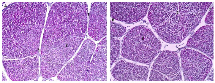
The objective of this study was to establish the morphological changes in the structure of Mediterranean mussel (Mytilus galloprovincialis) after frozen storage. Two hundred Mediterranean mussels (M. galloprovincialis) were collected from the Black Sea coastal waters. Forty mussels were subjected to histological analysis in fresh state. The remaining 160 mussels were divided into 4 groups and slowly frozen in a conventional freezer at −18 ℃ and subsequently stored at the same temperature for 3, 6, 9 and 12 months, respectively. The histological assessment of posterior adductor muscle and foot found a change in their morphological profile and overall structure. The fewest changes in the histostructure were recorded after a 3-month period and the most after a 12-month period of storage in frozen state. The results from that study can be used as an unambiguous marker in selecting optimum conditions for storage of mussels in frozen state.

References

[1]	Subramaniam T, Lee HJ, Jeung HD, et al. (2021) Report on the annual gametogenesis and tissue biochemical composition in the Gray mussel, Crenomytilus grayanus (Dunker 1853) in the subtidal rocky bottom on the east coast of Korea. Ocean Sci J 56: 424–433. https://doi.org/10.1007/s12601-021-00042-y doi: 10.1007/s12601-021-00042-y
[2]	Fitori A, Ishag IA, Masoud AN, et al. (2021) Assessment of some heavy metals using sediments and bivalvia (Mytilus galloprovincialis) samples collected from Tobruk coast. Sci J Fac Sci-Sirte Univ 1: 25–31. https://doi.org/10.37375/sjfssu.v1i2.79 doi: 10.37375/sjfssu.v1i2.79
[3]	Czech A, Grela ER, Ognik K (2015) Effect of frying on nutrients content and fatty acid composition of muscles of selected freezing seafoods. J Food Nutr Res 3: 9–14. https://doi.org/10.12691/jfnr-3-1-2 doi: 10.12691/jfnr-3-1-2
[4]	Tan K, Zhang HK, Li SK, et al. (2022) Lipid nutritional quality of marine and freshwater bivalves and their aquaculture potential. Crit Rev Food Sci Nutr 62: 6990–7014. https://doi.org/10.1080/10408398.2021.1909531 doi: 10.1080/10408398.2021.1909531
[5]	Gurdal AA, Caglak E (2021) Investigation of nutritional, some quality changes of mussels covered with edible films prepared using extracts of persimmon, Cherry Laurel and Likapa. Fresenius Environ Bull 30: 1823–1836.
[6]	Afsa S, De Marco G, Giannetto A, et al. (2022) Histological endpoints and oxidative stress transcriptional responses in the Mediterranean mussel Mytilus galloprovincialis exposed to realistic doses of salicylic acid. Environ Toxicol Pharmacol 92: 103855. https://doi.org/10.1016/j.etap.2022.103855 doi: 10.1016/j.etap.2022.103855
[7]	Peycheva K, Panayotova V, Stancheva R, et al. (2022) Effect of steaming on chemical composition of Mediterranean mussel (Mytilus galloprovincialis): Evaluation of potential risk associated with human consumption. Food Sci Nutr 10: 3052–3061. https://doi.org/10.1002/fsn3.2903 doi: 10.1002/fsn3.2903
[8]	Tan MT, Ye JX, Chu YM, et al. (2021) The effects of ice crystal on water properties and protein stability of large yellow croaker (Pseudosciaena crocea). Int J Refrig 130: 242–252. https://doi.org/10.1016/j.ijrefrig.2021.05.040 doi: 10.1016/j.ijrefrig.2021.05.040
[9]	Zhu SC, Yu HJ, Chen X, et al. (2021) Dual cryoprotective strategies for ice-binding and stabilizing of frozen seafood: A review. Trends Food Sci Technol 111: 223–232. https://doi.org/10.1016/j.tifs.2021.02.069 doi: 10.1016/j.tifs.2021.02.069
[10]	Lee S, Jo K, Jeong HG, et al. (2022) Freezing-induced denaturation of myofibrillar proteins in frozen meat. Crit Rev Food Sci Nutr, 1–18. https://doi.org/10.1080/10408398.2022.2116557 doi: 10.1080/10408398.2022.2116557
[11]	Al-Jeddawi W, Dawson P (2022) The effect of frozen storage on the quality of Atlantic Salmon. J Food Sci Nutr Res 5: 552–569. https://doi.org/10.26502/jfsnr.2642-11000098 doi: 10.26502/jfsnr.2642-11000098
[12]	Gao YP, Jiang HL, Lv DD, et al. (2021) Shelf-life of half-shell mussel (Mytilus edulis) as affected by pullulan, acidic electrolyzed water, and stable chlorine dioxide combined ice-glazing during frozen storage. Foods 10: 1896. https://doi.org/10.3390/foods10081896 doi: 10.3390/foods10081896
[13]	Tian J, Walayat N, Ding YT, et al. (2022) The role of trifunctional cryoprotectants in the frozen storage of aquatic foods: Recent developments and future recommendations. Compr Rev Food Sci Food Saf 21: 321–339. https://doi.org/10.1111/1541-4337.12865 doi: 10.1111/1541-4337.12865
[14]	Bardales JR, Cascallana JL, Villamarín A (2011) Differential distribution of cAMP-dependent protein kinase isoforms in various tissues of the bivalve mollusc Mytilus galloprovincialis. Acta Histochem 113: 743–748. https://doi.org/10.1016/j.acthis.2010.11.002 doi: 10.1016/j.acthis.2010.11.002
[15]	Cappello T, Maisano M, Mauceri A, et al. (2017) ¹ H NMR-based metabolomics investigation on the effects of petrochemical contamination in posterior adductor muscles of caged mussel Mytilus galloprovincialis. Ecotoxicol Environ Saf 142: 417–422. https://doi.org/10.1016/j.ecoenv.2017.04.040 doi: 10.1016/j.ecoenv.2017.04.040
[16]	Castro-Claros JD, Checa A, Lucena C, et al. (2021) Shell-adductor muscle attachment and Ca²⁺ transport in the bivalves Ostrea stentina and Anomia ephippium. Acta Biomater 120: 249–262. https://doi.org/10.1016/j.actbio.2020.09.053 doi: 10.1016/j.actbio.2020.09.053
[17]	Mediodia DP, Santander-de Leon SMS, Añasco N, et al. (2017) Shell Morphology and Anatomy of the Philippine Charru Mussel Mytella charruana (d'Orbigny 1842). Asian Fish Sci 30: 185–194. https://doi.org/10.33997/j.afs.2017.30.3.004 doi: 10.33997/j.afs.2017.30.3.004
[18]	Yamada A, Yoshio M, Nakamura A, et al. (2004) Protein phosphatase 2B dephosphorylates twitchin, initiating the catch state of invertebrate smooth muscle. J Biol Chem 279: 40762–40768. https://doi.org/10.1074/jbc.M405191200 doi: 10.1074/jbc.M405191200
[19]	McElwain A, Bullard SA (2014) Histological atlas of freshwater mussels (Bivalvia, Unionidae): Villosa nebulosa (Ambleminae: Lampsilini), Fusconaia cerina (Ambleminae: Pleurobemini) and Strophitus connasaugaensis (Unioninae: Anodontini). Malacologia 57: 99–239. https://doi.org/10.4002/040.057.0104 doi: 10.4002/040.057.0104
[20]	Simone LRL (2019) Modifications in adductor muscles in bivalves. Malacopedia 2: 1–12.
[21]	Vitellaro-Zuccarello L, De Biasi S, Amadeo A (1990) Immunocytochemical demonstration of neurotransmitters in the nerve plexuses of the foot and the anterior byssus retractor muscle of the mussel, Mytilus galloprovincialis. Cell Tissue Res 261: 467–476. https://doi.org/10.1007/BF00313525 doi: 10.1007/BF00313525
[22]	Balamurugan S, Subramanian P (2021) Histopathology of the foot, gill and digestive gland tissues of freshwater mussel, Lamellidens marginalis exposed to oil effluent. Austin J Environ Toxicol 7: 1033. https://doi.org/10.26420/austinjenvirontoxicol.2021.1033 doi: 10.26420/austinjenvirontoxicol.2021.1033
[23]	Lee JS, Lee YG, Park JJ, et al. (2012) Microanatomy and ultrastructure of the foot of the infaunal bivalve Tegillarca granosa (Bivalvia: Arcidae). Tissue Cell 44: 316–324. https://doi.org/10.1016/j.tice.2012.04.010 doi: 10.1016/j.tice.2012.04.010
[24]	Radwan EH, Saad GA, Hamed SSh (2016) Ultrastructural study on the foot and the shell of the oyster Pinctada radiata (leach, 1814), (Bivalvia Petridae). J Biosci Appl Res 2: 274–282. doi: 10.21608/jbaar.2016.107548
[25]	Angane M, Gupta S, Fletcher GC, et al. (2020) Effect of air blast freezing and frozen storage on Escherichia coli survival, n-3 polyunsaturated fatty acid concentration and microstructure of Greenshell^TM mussels. Food Control 115: 107284. https://doi.org/10.1016/j.foodcont.2020.107284 doi: 10.1016/j.foodcont.2020.107284
[26]	Park JJ, Lee JS, Lee YG, et al. (2012) Micromorphology and Ultrastructure of the Foot of the Equilateral Venus Gomphina veneriformis (Bivalvia: Veneridae). CellBio 1: 11–16. https://doi.org/10.4236/cellbio.2012.11002 doi: 10.4236/cellbio.2012.11002
[27]	Mohamed AS, Bin Dajem S, Al-Kahtani M, et al. (2021) Silver/chitosan nanocomposites induce physiological and histological changes in freshwater bivalve. J Trace Elem Med Biol 65: 126719. https://doi.org/10.1016/j.jtemb.2021.126719 doi: 10.1016/j.jtemb.2021.126719
[28]	Parisi MG, Baranzini N, Dara M, et al. (2022) AIF-1 and RNASET2 are involved in the inflammatory response in the Mediterranean mussel Mytilus galloprovincialis following Vibrio infection. Fish Shellfish Immun 127: 109–118. https://doi.org/10.1016/j.fsi.2022.06.010 doi: 10.1016/j.fsi.2022.06.010
[29]	Parisi MG, Maisano M, Cappello T, et al. (2019) Responses of marine mussel Mytilus galloprovincialis (Bivalvia: Mytilidae) after infection with the pathogen Vibrio splendidus. Comp Biochem Phys C 221: 1–9. https://doi.org/10.1016/j.cbpc.2019.03.005 doi: 10.1016/j.cbpc.2019.03.005
[30]	Sheir SK, Handy RD, Galloway TS (2010) Tissue injury and cellular immune responses to mercuric chloride exposure in the common mussel Mytilus edulis: Modulation by lipopolysaccharide. Ecotoxicol Environ Saf 73: 1338–1344. https://doi.org/10.1016/j.ecoenv.2010.01.014 doi: 10.1016/j.ecoenv.2010.01.014
[31]	Al-Subiai SN, Moody AJ, Mustafa SA, et al. (2011) A multiple biomarker approach to investigate the effects of copper on the marine bivalve mollusc, Mytilus edulis. Ecotoxicol Environ Saf 74: 1913–1920. https://doi.org/10.1016/j.ecoenv.2011.07.012 doi: 10.1016/j.ecoenv.2011.07.012
[32]	Nieto-Ortega S, Melado-Herreros Á, Foti G, et al. (2021) Rapid differentiation of unfrozen and frozen-thawed tuna with non-destructive methods and classification models: Bioelectrical impedance analysis (BIA), Near-infrared spectroscopy (NIR) and Time domain reflectometry (TDR). Foods 11: 55. https://doi.org/10.3390/foods11010055 doi: 10.3390/foods11010055
[33]	Yang SB, Hu YQ, Takaki K, et al. (2021) Effect of water ice-glazing on the quality of frozen swimming crab (Portunus trituberculatus) by liquid nitrogen spray freezing during frozen storage. Int J Refrig 131: 1010–1015. https://doi.org/10.1016/j.ijrefrig.2021.06.035 doi: 10.1016/j.ijrefrig.2021.06.035
[34]	Noomhorm A, Vongsawasdi P (2004) Freezing shellfish, In: Hui YH, Legarretta IG, Lim MH, et al. (Eds.), Handbook of frozen foods, New York: Marcel Dekker, 309–324.
[35]	Stella R, Mastrorilli E, Pretto T, et al. (2022) New strategies for the differentiation of fresh and frozen/thawed fish: Non-targeted metabolomics by LC-HRMS (part B). Food Control 132: 108461. https://doi.org/10.1016/j.foodcont.2021.108461 doi: 10.1016/j.foodcont.2021.108461
[36]	Tinacci L, Armani A, Guidi A, et al. (2018) Histological discrimination of fresh and frozen/thawed fish meat: European hake (Merluccius merluccius) as a possible model for white meat fish species. Food Control 92: 154–161. https://doi.org/10.1016/j.foodcont.2018.04.056 doi: 10.1016/j.foodcont.2018.04.056
[37]	Tinacci L, Armani A, Scardino G, et al. (2020) Selection of histological parameters for the development of an analytical method for discriminating fresh and frozen/thawed common octopus (Octopus vulgaris) and preventing frauds along the seafood chain. Food Anal Methods 13: 2111–2127. https://doi.org/10.1007/s12161-020-01825-0 doi: 10.1007/s12161-020-01825-0
[38]	Furnesvik L, Erkinharju T, Hansen M, et al. (2022) Evaluation of histological post-mortem changes in farmed Atlantic salmon (Salmo salar L.) at different time intervals and storage temperatures. J Fish Dis 45: 1571–1580. https://doi.org/10.1111/jfd.13681 doi: 10.1111/jfd.13681
[39]	Bouchendhomme T, Soret M, Devin A, et al. (2022) Differentiating between fresh and frozen-thawed fish fillets by mitochondrial permeability measurement. Food Control 141: 109197. https://doi.org/10.1016/j.foodcont.2022.109197 doi: 10.1016/j.foodcont.2022.109197
[40]	Shafieipour A, Sami M (2015) The effect of different thawing methods on chemical properties of frozen pink shrimp (Penaeus duorarum). Iran J Vet Med 9: 1–6. https://doi.org/10.22059/ijvm.2015.53226 doi: 10.22059/ijvm.2015.53226
[41]	Anderssen KE, Kranz M, Syed S, et al. (2022) Diffusion tensor imaging for spatially-resolved characterization of muscle fiber structure in seafood. Food Chem 380: 132099. https://doi.org/10.1016/j.foodchem.2022.132099 doi: 10.1016/j.foodchem.2022.132099
[42]	Zhang LH, Zhang M, Mujumdar AS (2021) Technological innovations or advancement in detecting frozen and thawed meat quality: A review. Crit Rev Food Sci Nutr, 1–17. https://doi.org/10.1080/10408398.2021.1964434 doi: 10.1080/10408398.2021.1964434

Reader Comments

Your name:*

Email:*
© 2023 the Author(s), licensee AIMS Press. This is an open access article distributed under the terms of the Creative Commons Attribution License (http://creativecommons.org/licenses/by/4.0)