Benefits of biochar application on environment conservation and agricultural production have been widely studied. However, few studies were focused on root development. The objective of this study covered root and shoot development, yield, and soil properties associated with exposure of Oryza glaberrima rice during the early reproductive stage to drought stress in rice-husk amended soil. The biochar was amended at a rate of 10.5 g pot-1, equivalent to 3 ton ha-1. Biochar-amended and non-amended plants were exposed to drought stress after the panicles had visibly emerged in all plant populations. Biochar application caused less restriction on root elongation, volume, and surface area during water stress conditions. Enhanced root development was primarily associated with improvement in water status and chemical properties in biochar-amended soil. Soil chemical properties improved, including increased soil pH, available P, cation exchange capacity, and exchangeable Mg. Under drought stress conditions, shoot growth was more sensitive than root growth, as indicated by the significant reduction of stem dry weight (SDW) and leaf dry weight (LDW). Fine roots in biochar-amended soil were longer than those in non-amended soil. In general, Biochar application enable the O. glaberrima rice to maintain yield under drought stress condition.
Citation: Kartika Kartika, Jun-Ichi Sakagami, Benyamin Lakitan, Shin Yabuta, Isao Akagi, Laily Ilman Widuri, Erna Siaga, Hibiki Iwanaga, Arinal Haq Izzawati Nurrahma. Rice husk biochar effects on improving soil properties and root development in rice (Oryza glaberrima Steud.) exposed to drought stress during early reproductive stage[J]. AIMS Agriculture and Food, 2021, 6(2): 737-751. doi: 10.3934/agrfood.2021043
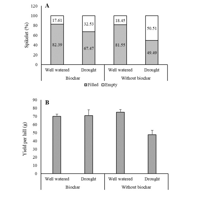
Benefits of biochar application on environment conservation and agricultural production have been widely studied. However, few studies were focused on root development. The objective of this study covered root and shoot development, yield, and soil properties associated with exposure of Oryza glaberrima rice during the early reproductive stage to drought stress in rice-husk amended soil. The biochar was amended at a rate of 10.5 g pot-1, equivalent to 3 ton ha-1. Biochar-amended and non-amended plants were exposed to drought stress after the panicles had visibly emerged in all plant populations. Biochar application caused less restriction on root elongation, volume, and surface area during water stress conditions. Enhanced root development was primarily associated with improvement in water status and chemical properties in biochar-amended soil. Soil chemical properties improved, including increased soil pH, available P, cation exchange capacity, and exchangeable Mg. Under drought stress conditions, shoot growth was more sensitive than root growth, as indicated by the significant reduction of stem dry weight (SDW) and leaf dry weight (LDW). Fine roots in biochar-amended soil were longer than those in non-amended soil. In general, Biochar application enable the O. glaberrima rice to maintain yield under drought stress condition.

| [1] | Widuri LI, Lakitan B, Sodikin E, et al. (2018) Shoot and root growth in common bean (Phaseolus vulgaris L.) exposed to gradual drought stress. Agrivita 40: 442-449. |
| [2] | Lakitan B, Hadi B, Herlinda S, et al. (2018) Recognizing farmers' practices and constraints for intensifying rice production at Riparian Wetlands in Indonesia. NJAS-Wageningen J Life Sci 85: 10-20. |
| [3] | Lakitan B, Widuri LI, Meihana M, et al. (2017) Simplifying procedure for a non-destructive, inexpensive, yet accurate trifoliate leaf area estimation in snap bean (Phaseolus vulgaris). J Appl Hort 19: 15-21. |
| [4] | Kartika K, Lakitan B, Sanjaya N, et al. (2018a) Internal versus edge row comparison in Jajar legowo 4: 1 rice planting pattern at different frequency of fertilizer applications. Agrivita 40: 222-232. |
| [5] | Yang J, Zhang J (2006) Grain filling of cereals under soil drying. New Phytol 169: 223-236. |
| [6] | Keshavarz AR, Hashemi M, DaCosta M, et al. (2016) Biochar application and drought stress effects on physiological characteristics of Silybum marianum. Commun Soil Sci Plant Anal 47: 743-752. |
| [7] | Yamato M, Okimori Y, Wibowo IF, et al. (2006). Effects of the application of charred bark of Acacia mangium on the yield of maize, cowpea and peanut, and soil chemical properties in South Sumatra, Indonesia. Soil Sci Plant Nutr 52: 489-495. |
| [8] | Dunnigan L, Ashman PJ, Zhang X, et al. (2018) Production of biochar from rice husk: Particulate emissions from the combustion of raw pyrolysis volatiles. J Clean Prod 172: 1639-1645. |
| [9] | Abrishamkesh S, Gorji M, Asadi H, et al. (2015) Effects of rice husk biochar application on the properties of alkaline soil and lentil growth. Plant Soil & Environ 61: 475-482. |
| [10] | Kartika K, Lakitan B, Wijaya A, et al. (2018b) Effects of particle size and application rate of rice-husk biochar on chemical properties of tropical wetland soil, rice growth and yield. Aust J Crop Sci 12: 817-826. |
| [11] | Liu S, Meng J, Jiang L, et al. (2017) Rice husk biochar impacts soil phosphorous availability, phosphatase activities and bacterial community characteristics in three different soil types. Appl Soil Ecol 116: 12-22. |
| [12] | Brennan A, Jiménez EM, Puschenreiter M, et al. (2014) Effects of biochar amendment on root traits and contaminant availability of maize plants in a copper and arsenic impacted soil. Plant Soil 379: 351-360. |
| [13] | Vanek SJ, Lehmann J (2015) Phosphorus availability to beans via interactions between mycorrhizas and biochar. Plant Soil 395: 105-123. |
| [14] | Xiang Y, Deng Q, Duan H, et al. (2017) Effects of biochar application on root traits: A meta-analysis. GCB Bioenergy 9: 1563-1572. |
| [15] | Kim Y, Chung YS, Lee E, et al. (2020) Root response to drought stress in rice (Oryza sativa L.). Int J Mol Sci 21: 122. |
| [16] | Sarla N, Swamy BPM (2005) Oryza glaberrima: A source for the improvement of Oryza sativa. Curr Sci 89: 955-963. |
| [17] | Kartika K, Sakagami JI, Lakitan B, et al. (2020) Morpho-physiological response of Oryza glaberrima to gradual soil drying. Rice Science 27: 67-74. |
| [18] | Lu SG, Sun FF, Zong YT (2014) Effect of rice husk biochar and coal fly ash on some physical properties of expansive clayey soil (Vertisol). Catena 114: 37-44. |
| [19] | Akhtar SS, Andersen MN, Liu F (2015) Biochar mitigates salinity stress in potato. J Agron Crop Sci 201: 368-378. |
| [20] | Foster EJ, Hansen N, Wallenstein M, et al. (2016) Biochar and manure amendments impact soil nutrients and microbial enzymatic activities in a semi-arid irrigated maize cropping system. Agric Ecosyst Environ 233: 404-414. |
| [21] | Asai H, Samson BK, Stephan HM, et al. (2009) Biochar amendment techniques for upland rice production in Northern Laos. 1. Soil physical properties, leaf SPAD and grain yield. Field Crop Res 111: 81-84. |
| [22] | Artiola JF, Rasmussen C, Freitas R (2012) Effects of a biochar-amended alkaline soil on the growth of romaine lettuce and bermudagrass. Soil Sci 177: 561-570. |
| [23] | Abel S, Peters A, Trinks S, et al. (2013) Impact of biochar and hydrochar addition on water retention and water repellency of sandy soil. Geoderma 202: 183-191. |
| [24] | Novak JM, Busscher WJ, Watts DW, et al. (2012) Biochars impact on soil-moisture storage in an ultisol and two aridisols. Soil Sci 177: 310-320. |
| [25] | Laird DA (2008) The charcoal vision: A win-win-win scenario for simultaneously producing bioenergy, permanently sequestering carbon, while improving soil and water quality. Agron J 100: 178-181. |
| [26] | Sohi SP, Krull E, Lopez-Capel E, et al. (2010) A review of biochar and its use and function in soil. Adv Agronomy 105: 47-82. |
| [27] | Van Zwieten L, Kimber S, Morris S, et al. (2010) Effects of biochar from slow pyrolysis of papermill waste on agronomic performance and soil fertility. Plant Soil 327: 235-246. |
| [28] | Obia A, Cornelissen G, Mulder J, et al. (2015) Effect of soil pH increase by biochar on NO, N2O and N2 production during denitrification in acid soils. PLoS One 10: e0138781. |
| [29] | Liang B, Lehmann J, Solomon D, et al. (2006) Black carbon increases cation exchange capacity in soils. Soil Sci Soc Amer J 70: 1719-1730. |
| [30] | Jien SH, Wang CS (2013) Effects of biochar on soil properties and erosion potential in a highly weathered soil. Catena 110: 225-233. |
| [31] | Cui HJ, Wang MK, Fu ML, et al. (2011) Enhancing phosphorus availability in phosphorus-fertilized zones by reducing phosphate adsorbed on ferrihydrite using rice straw-derived biochar. J Soil Sediment 11: 1135-1141. |
| [32] | Li D, Shi X, Zhao Y, et al. (2016) Rice-husk biochar improved soil properties and wheat yield on an acidified purple soil. In: Kim YH, The 5th International Conference on Civil, Architectural and Hydraulic Engineering (ICCAHE), Dordrecht, The Netherlands: Atlantis Press, 294-302. |
| [33] | Mahajan S, Tuteja N (2005) Cold, salinity and drought stresses: An overview. Arch Biochem Biophys 444: 139-158. |
| [34] | Widuri LI, Lakitan B, Hasmeda M, et al. (2017) Relative leaf expansion rate and other leaf-related indicators for detection of drought stress in chili pepper (Capsicum annuum L.). Aust J Crop Sci 11: 1617-1625. |
| [35] | Sakagami JI (2012) Submergence tolerance of rice species Oryza glaberrima Steud. In: Najafpour M, Applied Photosynthesis, Germany: Books on Demand, 353-364. |
| [36] | Bañon S, Fernandez JA, Franco JA, et al. (2004) Effects of water stress and night temperature preconditioning on water relations and morphological and anatomical changes of Lotus creticus plants. Sci Hortic 101: 333-342. |
| [37] | Comas LH, Mueller KE, Taylor LL, et al. (2012) Evolutionary patterns and biogeochemical significance of angiosperm root traits. Int J Plant Sci 173: 584-595. |
| [38] | Dien DC, Yamakawa T, Mochizuki T, et al. (2017) Dry weight accumulation, root plasticity, and stomatal conductance in rice (Oryza sativa L.) varieties under drought stress and re-watering conditions. Amer J Plant Sci 8: 3189-3206. |
| [39] | Wasaya A, Zhang X, Fang Q, et al. (2018) Root phenotyping for drought tolerance: A review. Agronomy 8: 241-260. |
| [40] | Lakitan B, Alberto A, Lindiana L, et al. (2018b) The benefits of biochar on rice growth and yield in tropical riparian wetland, South Sumatra, Indonesia. Chiang Mai Univ J Nat Sci 17: 111-126. |
| [41] | Cornelissen G, Martinsen V, Shitumbanuma V, et al. (2013). Biochar effect on maize yield and soil characteristics in five conservation farming sites in Zambia. Agronomy, 3: 256-274. |
Figures(5) / Tables(3)

Kartika Kartika, Jun-Ichi Sakagami, Benyamin Lakitan, Shin Yabuta, Isao Akagi, Laily Ilman Widuri, Erna Siaga, Hibiki Iwanaga, Arinal Haq Izzawati Nurrahma. Rice husk biochar effects on improving soil properties and root development in rice (Oryza glaberrima Steud.) exposed to drought stress during early reproductive stage[J]. AIMS Agriculture and Food, 2021, 6(2): 737-751. doi: 10.3934/agrfood.2021043


 DownLoad: