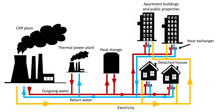
Intelligent district heating control requires knowing the customers' past behavior and predicting their future needs. This can reduce peak energy use, optimizing energy production, accurate billing, and reducing fraud. Clustering has been used for analyzing large-scale building operational data and recognizing consumption profiles. In this work, we analyze the heat consumption profiles of district heat customers in Kuopio, Finland. We constructed two consumption profiles of their average hourly use: one for weekdays, and one for weekends. Clustering is then used to construct four consumption profiles. These profiles can be used for intelligent control, prediction of future use, and to recognize abnormal use behavior. The latter can be the first indication of a problem like heat leaking, which can prevent possible water damage.
Citation: Vili Lavikainen, Pasi Fränti. Clustering district heating customers based on load profiles[J]. Applied Computing and Intelligence, 2024, 4(2): 269-281. doi: 10.3934/aci.2024016
Intelligent district heating control requires knowing the customers' past behavior and predicting their future needs. This can reduce peak energy use, optimizing energy production, accurate billing, and reducing fraud. Clustering has been used for analyzing large-scale building operational data and recognizing consumption profiles. In this work, we analyze the heat consumption profiles of district heat customers in Kuopio, Finland. We constructed two consumption profiles of their average hourly use: one for weekdays, and one for weekends. Clustering is then used to construct four consumption profiles. These profiles can be used for intelligent control, prediction of future use, and to recognize abnormal use behavior. The latter can be the first indication of a problem like heat leaking, which can prevent possible water damage.

| [1] | Energiateollisuus ry, Energy year 2021—electricity (Finnish), Finnish Energy, 2022. Available from: https://energia.fi/en/statistics/energy-year-2021-electricity/. |
| [2] | Motiva, District heating (Finnish), Motiva Oy, 2022. Available from: https://www.motiva.fi/koti_ja_asuminen/rakentaminen/lammitysjarjestelman_valinta/lammitysmuodot/kaukolampo. |
| [3] |
K. Skytte, O. Olsen, Regulatory barriers for flexible coupling of the Nordic power and district heating markets, Proceedings of 13th International Conference on the European Energy Market (EEM), 2016, 1–5. https://doi.org/10.1109/EEM.2016.7521319 doi: 10.1109/EEM.2016.7521319

|
| [4] |
G. Schweiger, J. Rantzer, K. Ericsson, P. Lauenburg, The potential of power-to-heat in Swedish district heating systems, Energy, 137 (2017), 661–669. https://doi.org/10.1016/j.energy.2017.02.075 doi: 10.1016/j.energy.2017.02.075
|
| [5] |
M. Razmara, G. Bharati, D. Hanover, M. Shahbakhti, S. Paudyal, R. Robinett Ⅲ, Building-to-grid predictive power flow control for demand response and demand flexibility programs, Appl. Energ., 203 (2017), 128–141. https://doi.org/10.1016/j.apenergy.2017.06.040 doi: 10.1016/j.apenergy.2017.06.040
|
| [6] |
H. Li, S. Wang, Challenges in smart low-temperature district heating development, Energy Procedia, 61 (2014), 1472–1475. https://doi.org/10.1016/j.egypro.2014.12.150 doi: 10.1016/j.egypro.2014.12.150
|
| [7] |
U. Persson, S. Werner, Heat distribution and the future competitiveness of district heating, Appl. Energ., 88 (2011), 568–576. https://doi.org/10.1016/j.apenergy.2010.09.020 doi: 10.1016/j.apenergy.2010.09.020
|
| [8] |
H. Gadd, S. Werner, Achieving low return temperatures from district heating substations, Appl. Energ., 136 (2014), 59–67. https://doi.org/10.1016/j.apenergy.2014.09.022 doi: 10.1016/j.apenergy.2014.09.022
|
| [9] | S. Werner, District heating and cooling, In: Reference module in earth systems and environmental sciences, 2013, 1–7. https://doi.org/10.1016/B978-0-12-409548-9.01094-0 |
| [10] |
S. Nilsson, C. Reidhav, K. Lygnerud, S. Werner, Sparse district-heating in Sweden, Appl. Energ., 85 (2008), 555–564. https://doi.org/10.1016/j.apenergy.2007.07.011 doi: 10.1016/j.apenergy.2007.07.011
|
| [11] |
C. Reidhav, S. Werner, Profitability of sparse district heating, Appl. Energ., 85 (2008), 867–877. https://doi.org/10.1016/j.apenergy.2008.01.006 doi: 10.1016/j.apenergy.2008.01.006
|
| [12] |
F. Levihn, CHP and heat pumps to balance renewable power production: lessons from the district heating network in Stockholm, Energy, 137 (2017), 670–678. https://doi.org/10.1016/j.energy.2017.01.118 doi: 10.1016/j.energy.2017.01.118
|
| [13] |
M. Sameti, F. Haghighat, Optimization approaches in district heating and cooling thermal network, Energ. Buildings, 140 (2017), 121–130. https://doi.org/10.1016/j.enbuild.2017.01.062 doi: 10.1016/j.enbuild.2017.01.062
|
| [14] |
G. Mbiydzenyuy, S. Nowaczyk, H. Knutsson, D. Vanhoudt, J. Brage, E. Calikus, Opportunities for machine learning in district heating, Appl. Sci., 11 (2021), 6112. https://doi.org/10.3390/app11136112 doi: 10.3390/app11136112
|
| [15] |
S. Darby, Smart metering: what potential for householder engagement? Build. Res. Inf., 38 (2010), 442–457. https://doi.org/10.1080/09613218.2010.492660 doi: 10.1080/09613218.2010.492660
|
| [16] |
E. Calikus, S. Nowaczyk, A. Sant'Anna, H. Gadd, S. Werner, A data-driven approach for discovering heat load patterns in district heating, Appl. Energ., 252 (2019), 113409. https://doi.org/10.1016/j.apenergy.2019.113409 doi: 10.1016/j.apenergy.2019.113409
|
| [17] |
A. Kipping, E. Trømborg, Modeling and disaggregating hourly electricity consumption in Norwegian dwellings based on smart meter data, Energ. Buildings, 118 (2016), 350–369. https://doi.org/10.1016/j.enbuild.2016.02.042 doi: 10.1016/j.enbuild.2016.02.042
|
| [18] |
M. Noussan, M. Jarre, A. Poggio, Real operation data analysis on district heating load patterns, Energy, 129 (2017), 70–78. https://doi.org/10.1016/j.energy.2017.04.079 doi: 10.1016/j.energy.2017.04.079
|
| [19] |
Z. Ma, H. Li, Q. Sun, C. Wang, A. Yan, F. Starfelt, Statistical analysis of energy consumption patterns on the heat demand of buildings in district heating systems, Energ. Buildings, 85 (2014), 464–472. https://doi.org/10.1016/j.enbuild.2014.09.048 doi: 10.1016/j.enbuild.2014.09.048
|
| [20] | L. Koskelainen, R. Saarela, K. Sipilä, Kaukolämmön käsikirja (Finnish), Helsinki: Energiateollisuus ry, 2006. |
| [21] |
Y. Lu, Z. Tian, P. Peng, J. Niu, W. Li, H. Zhang, GMM clustering for heating load patterns in-depth identification and prediction model accuracy improvement of district heating system, Energ. Buildings, 190 (2019), 49–60. https://doi.org/10.1016/j.enbuild.2019.02.014 doi: 10.1016/j.enbuild.2019.02.014
|
| [22] |
Z. Yu, F. Haghighat, B. Fung, L. Zhou, A novel methodology for knowledge discovery through mining associations between building operational data, Energ. Buildings, 47 (2012), 430–440. https://doi.org/10.1016/j.enbuild.2011.12.018 doi: 10.1016/j.enbuild.2011.12.018
|
| [23] |
F. Xiao, C. Fan, Data mining in building automation system for improving building operational performance, Energ. Buildings, 75 (2014), 109–118. https://doi.org/10.1016/j.enbuild.2014.02.005 doi: 10.1016/j.enbuild.2014.02.005
|
| [24] |
A. Goia, C. May, G. Fusai, Functional clustering and linear regression for peak load forecasting, Int. J. Forecasting, 26 (2010), 700–711. https://doi.org/10.1016/j.ijforecast.2009.05.015 doi: 10.1016/j.ijforecast.2009.05.015
|
| [25] |
P. Duan, K. Xie, T. Guo, X. Huang, Short-term load forecasting for electric power systems using the PSO-SVR and FCM clustering techniques, Energies, 4 (2011), 173–184. https://doi.org/10.3390/en4010173 doi: 10.3390/en4010173
|
| [26] | Ediel, Message handbook for Ediel implementation guide for metered services consumption report, Ediel forum, 2010. Available from: https://ediel.org/wp-content/uploads/2019/02/MSCONS-24E-20100215.pdf. |
| [27] | FMI, Ilmatieteen laitoksen avoin data ja lähdekoodi, Finnish Meteorological Institute, 2023. Available from: https://www.ilmatieteenlaitos.fi/avoin-data. |
| [28] |
C. Wang, Y. Du, H. Li, F. Wallin, G. Min, New methods for clustering district heating users based on consumption patterns, Appl. Energ., 251 (2019), 113373. https://doi.org/10.1016/j.apenergy.2019.113373 doi: 10.1016/j.apenergy.2019.113373
|
| [29] |
P. Fränti, S. Sieranoja, How much can k-means be improved by using better initialization and repeats? Pattern Recogn., 93 (2019), 95–112. https://doi.org/10.1016/j.patcog.2019.04.014 doi: 10.1016/j.patcog.2019.04.014
|
| [30] |
P. Fränti, Efficiency of random swap clustering, J. Big Data, 5 (2018), 13. https://doi.org/10.1186/s40537-018-0122-y doi: 10.1186/s40537-018-0122-y
|
| [31] |
S. Sieranoja, P. Fränti, Adapting k-means for graph clustering, Knowl. Inf. Syst., 64 (2022), 115–142. https://doi.org/10.1007/s10115-021-01623-y doi: 10.1007/s10115-021-01623-y
|
| [32] |
M. Rezaei, P. Fränti, K-sets and k-swaps algorithms for clustering sets, Pattern Recogn., 139 (2023), 109454. https://doi.org/10.1016/j.patcog.2023.109454 doi: 10.1016/j.patcog.2023.109454
|
| [33] |
J. Paparrizos, L. Gravano, Fast and accurate time-series clustering, ACM Trans. Database Syst., 42 (2017), 8. https://doi.org/10.1145/3044711 doi: 10.1145/3044711
|
| [34] |
P. Fränti, S. Sieranoja, K-means properties on six clustering benchmark datasets, Appl. Intell., 48 (2018), 4743–4759. https://doi.org/10.1007/s10489-018-1238-7 doi: 10.1007/s10489-018-1238-7
|
| [35] | R. Tavenard, J. Faouzi, G. Vandewiele, F. Divo, G. Androz, C. Holtz, et al., Tslearn, a machine learning toolkit for time series data, J. Mach. Learn. Res., 21 (2020), 1–6. |
| [36] |
T. Caliński, J. Harabasz, A dendrite method for cluster analysis, Commun. Stat., 3 (1974), 1–27. https://doi.org/10.1080/03610927408827101 doi: 10.1080/03610927408827101
|
| [37] | D. Davies, D. Bouldin, A cluster separation measure, IEEE Trans. Pattern Anal., PAMI-1 (1979), 224–227. https://doi.org/10.1109/TPAMI.1979.4766909 |
| [38] |
P. Rousseeuw, Silhouettes: a graphical aid to the interpretation and validation of cluster analysis, J. Comput. Appl. Math., 20 (1987), 53–65. https://doi.org/10.1016/0377-0427(87)90125-7 doi: 10.1016/0377-0427(87)90125-7
|
| [39] |
R. Tibshirani, G. Walther, T. Hastie, Estimating the number of clusters in a data set via the gap statistic, J. R. Stat. Soc. B, 63 (2001), 411–423. https://doi.org/10.1111/1467-9868.00293 doi: 10.1111/1467-9868.00293
|
| [40] |
Q. Zhao, P. Fränti, WB-index: a sum-of-squares based index for cluster validity, Data Knowl. Eng., 92 (2014), 77–89. https://doi.org/10.1016/j.datak.2014.07.008 doi: 10.1016/j.datak.2014.07.008
|
| [41] |
A. Javed, B. Lee, D. Rizzo, A benchmark study on time series clustering, Machine Learning with Applications, 1 (2020), 100001. https://doi.org/10.1016/j.mlwa.2020.100001 doi: 10.1016/j.mlwa.2020.100001
|


Figures(9) / Tables(2)
Vili Lavikainen, Pasi Fränti. Clustering district heating customers based on load profiles[J]. Applied Computing and Intelligence, 2024, 4(2): 269-281. doi: 10.3934/aci.2024016


 DownLoad: