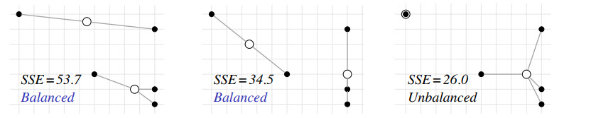
Loading [MathJax]/jax/output/SVG/jax.js
Research article

Balanced k-means revisited

  • Received: 06 October 2023 Accepted: 17 October 2023 Published: 27 October 2023
  • The k-means algorithm aims at minimizing the variance within clusters without considering the balance of cluster sizes. Balanced k-means defines the partition as a pairing problem that enforces the cluster sizes to be strictly balanced, but the resulting algorithm is impractically slow O(n3). Regularized k-means addresses the problem using a regularization term including a balance parameter. It works reasonably well when the balance of the cluster sizes is a mandatory requirement but does not generalize well for soft balance requirements. In this paper, we revisit the k-means algorithm as a two-objective optimization problem with two goals contradicting each other: to minimize the variance within clusters and to minimize the difference in cluster sizes. The proposed algorithm implements a balance-driven variant of k-means which initially only focuses on minimizing the variance but adds more weight to the balance constraint in each iteration. The resulting balance degree is not determined by a control parameter that has to be tuned, but by the point of termination which can be precisely specified by a balance criterion.

    Citation: Rieke de Maeyer, Sami Sieranoja, Pasi Fränti. Balanced k-means revisited[J]. Applied Computing and Intelligence, 2023, 3(2): 145-179. doi: 10.3934/aci.2023008

    Related Papers:

    [1] Mikko I. Malinen, Pasi Fränti . All-pairwise squared distances lead to more balanced clustering. Applied Computing and Intelligence, 2023, 3(1): 93-115. doi: 10.3934/aci.2023006
    [2] Marko Niemelä, Mikaela von Bonsdorff, Sami Äyrämö, Tommi Kärkkäinen . Classification of dementia from spoken speech using feature selection and the bag of acoustic words model. Applied Computing and Intelligence, 2024, 4(1): 45-65. doi: 10.3934/aci.2024004
    [3] Le Li, Fei Wang . HBC: halo-based clustering using local comparative density. Applied Computing and Intelligence, 2024, 4(2): 164-183. doi: 10.3934/aci.2024010
    [4] Isaiah Kiprono Mutai, Kristof Van Laerhoven, Nancy Wangechi Karuri, Robert Kimutai Tewo . Using multiple linear regression for biochemical oxygen demand prediction in water. Applied Computing and Intelligence, 2024, 4(2): 125-137. doi: 10.3934/aci.2024008
    [5] Xu Ji, Fang Dong, Zhaowu Huang, Xiaolin Guo, Haopeng Zhu, Baijun Chen, Jun Shen . Edge-assisted multi-user millimeter-wave radar for non-contact blood pressure monitoring. Applied Computing and Intelligence, 2025, 5(1): 57-76. doi: 10.3934/aci.2025004
    [6] Hao Zhen, Yucheng Shi, Jidong J. Yang, Javad Mohammadpour Vehni . Co-supervised learning paradigm with conditional generative adversarial networks for sample-efficient classification. Applied Computing and Intelligence, 2023, 3(1): 13-26. doi: 10.3934/aci.2023002
    [7] Sheyda Ghanbaralizadeh Bahnemiri, Mykola Pnomarenko, Karen Eguiazarian . Iterative transfer learning with large unlabeled datasets for no-reference image quality assessment. Applied Computing and Intelligence, 2024, 4(2): 107-124. doi: 10.3934/aci.2024007
    [8] Pasi Fränti, Sami Sieranoja . Clustering accuracy. Applied Computing and Intelligence, 2024, 4(1): 24-44. doi: 10.3934/aci.2024003
    [9] Pasi Fränti, Olli Virmajoki . Optimal clustering by merge-based branch-and-bound. Applied Computing and Intelligence, 2022, 2(1): 63-82. doi: 10.3934/aci.2022004
    [10] Xian Wen Sim, Sie Long Kek, Sy Yi Sim . State estimation and optimal control of an inverted pendulum on a cart system with stochastic approximation approach. Applied Computing and Intelligence, 2023, 3(1): 79-92. doi: 10.3934/aci.2023005
  • The k-means algorithm aims at minimizing the variance within clusters without considering the balance of cluster sizes. Balanced k-means defines the partition as a pairing problem that enforces the cluster sizes to be strictly balanced, but the resulting algorithm is impractically slow O(n3). Regularized k-means addresses the problem using a regularization term including a balance parameter. It works reasonably well when the balance of the cluster sizes is a mandatory requirement but does not generalize well for soft balance requirements. In this paper, we revisit the k-means algorithm as a two-objective optimization problem with two goals contradicting each other: to minimize the variance within clusters and to minimize the difference in cluster sizes. The proposed algorithm implements a balance-driven variant of k-means which initially only focuses on minimizing the variance but adds more weight to the balance constraint in each iteration. The resulting balance degree is not determined by a control parameter that has to be tuned, but by the point of termination which can be precisely specified by a balance criterion.


    The clustering problem is to partition objects into separate groups (called clusters) so that objects within one cluster are more similar to each other than objects in different clusters [1]. Since the middle of the 20th century, thousands of algorithms addressing the clustering problem have been published [2].

    One of the most popular clustering algorithms is the k-means algorithm [2,3]. It was first proposed by [4] and [5]. This clustering algorithm aims to build k disjoint clusters such that the sum of squared distances between the data points and their representatives is minimized. The representatives, called centroids, are determined by the mean of the data points belonging to a cluster. As a distance function, the Euclidean distance is used. The number of clusters k has to be set by the user.

    Formally, if we have a data set consisting of n data points x1, x2, , xn, the task is to group these data points into k clusters such that the sum squared error (SSE)

    SSE=kj=1xipj||xicj||2 (1)

    is minimized, where pj denotes the set of data points assigned to the jth cluster and cj is the centroid of the jth cluster. This problem is NP-hard even for two clusters [6]. The k-means algorithm is a heuristic for this problem.

    The algorithm itself starts by initializing the centroid locations. This is followed by an assignment and update steps which are iterated until a convergence criterion is met. During the initialization, k cluster centroids are randomly selected from all data points. In the assignment step, each data point is assigned to the cluster whose centroid is closest. Formally, the assignment step can be written as

    pj={xi|argminj{1,,k}(||xicj||2)=j} for all j{1,,k}.

    In the update step, the centroids are updated by the mean of the data points assigned to the cluster. Formally,

    cj=1|pj|xipjxi for all j{1,,k},

    where |pj| denotes the number of data points assigned to the jth cluster. The assignment and update steps are repeated until the centroids do not change anymore.

    This algorithm is a heuristic not necessarily returning a global optimum [7]. Nevertheless, it returns a local optimum with respect to the SSE: the assignment step minimizes the SSE for a given set of centroids, while the update step minimizes the SSE for a given partition [7,8]. The running time of one iteration is linear in the number of data points n [9].

    Among the advantages of this algorithm are its simplicity, time complexity, and usability in a large area of subjects [9,10]. However, despite its popularity, it also involves some drawbacks like the strong dependence on the initial choice of the cluster centroids [10,11] or its limitation to hyperspherical shaped clusters [12]. Another drawback, on which we focus in this paper, is its inability to control the number of objects contained in each cluster. Especially in high dimensional space and if many clusters are desired, often very small clusters seem to appear even if the data itself has a balanced distribution [13].

    In this paper, we refer to a balanced clustering as a clustering that distributes the data points evenly between the clusters. More formally, to incorporate situations in which the number of data points n is not divisible by the number of clusters k, a balanced clustering requires that every cluster contains either nk or nk data points.

    In general, balanced clustering is a two-objective optimization problem pursuing two goals that contradict each other: On the one hand, the SSE should be minimized, and on the other hand, the difference in cluster sizes should be minimized. If we were just interested in minimizing the SSE, we could apply an ordinary clustering algorithm like k-means, and if we were only interested in balancing, we could simply divide the data points randomly into clusters of the same size [7,10]. Figure 1 demonstrates the case where minimizing the SSE with and without a balance constraint results in a different optimal clustering result.

    Figure 1.  Balance constraints can lead to a different clustering result. There are two balanced clusterings with different SSE values (left and middle) and one unconstrained clustering optimized for SSE (right).

    To optimize both aims, there exist two different approaches, hard-balanced, also called balance-constrained, and soft-balanced, also called balance-driven, clustering. Both approaches differ in the way they assess the two objectives. Hard-balanced clustering strictly requires cluster size balance, whereas the minimization of the SSE serves as a secondary criterion. Soft-balanced clustering considers the balance of the cluster sizes as an aim but not as a mandatory requirement. It intends to find a compromise between the two goals, e.g., by weighting them or by using a heuristic which minimizes the SSE but indirectly creates more balanced clusters than the standard k-means algorithm [7,8].

    In this paper, we propose a balanced clustering algorithm based on the k-means algorithm. Its main principle is an increasing penalty term, which is added to the assignment function of the k-means algorithm and favors objects to be assigned to smaller clusters. Because of the increasing penalty term, the resulting balance degree of a clustering is not determined by a rather non-intuitive parameter, but by the point of termination of the algorithm. In this way, the desired balance degree can be specified precisely. However, even if the algorithm has found a clustering with the desired balance degree, it may still be possible to improve the quality of the clustering (SSE) by iterating the algorithm further while keeping the last penalty term fixed.

    There are many applications for clustering that rely on a balanced distribution of the objects, i.e., a distribution in which every cluster contains exactly or approximately the same number of objects. Balanced clustering can be used in the division step of divide-and-conquer algorithms to provide equal-sized partitions [7]. In load balancing algorithms, balanced clustering can help to avoid unbalanced energy consumption in networking [8,14,15] or to balance the workload of salesmen in the multiple traveling salesmen problem [16]. In the clustering of documents, articles or photos. Also, in the creation of domain-specific ontologies, balanced clustering can improve the resulting hierarchies by generating a more balanced view of the objects to facilitate navigation and browsing [17]. In retail chains, balanced clustering can be used to segment customers into equal-sized groups to spend the same amount of marketing resources on each segment or to group similar products into categories of specified sizes to match units of shelf or floor space [17]. Cost function leading to more balanced cluster sizes was used in [18] to allow manual investigation of the content of the diagnosis clusters.

    A fast O(N1.5) time divide-and-conquer algorithm for planar minimum spanning tree (MST) in [19] assumed that the points are distributed equally among the clusters. However, this assumption does not hold if there is even a single large cluster, and the time complexity of the algorithm grows to O(N2). This can be easily avoided using a more balanced clustering algorithm where the worst-case behavior (with one very large cluster) is avoided. For MST, the quality of the clustering is not important as it is merely used as a tool to split the dataset in a meaningful way.

    Another example is a clustering-based TSP algorithm [20], which normally requires O(Nlog(N)) but has the worst-case complexity O(N2) in the same situation when one cluster is very large (rest containing only one node).

    The rest of the paper is organized as follows. We begin in Section 2 by summarizing the related work. In Section 3 we present the proposed algorithm. After demonstrating its main principle on a small exemplary data set, we focus on the magnitude of the penalty term and its computation. Further, we briefly consider its termination criterion and time complexity. Section 6 shows the results. We compare the proposed method to the regularized k-means algorithm by [8] and the balanced k-means algorithm by [7] on several data sets.

    We next review the existing approaches for balanced clustering. Approaches for hard-balanced clustering are reviewed in Section 2.1 and for soft-balanced clustering in Section 2.2, respectively.

    A popular approach to face this problem is to formulate the assignment step of the standard k-means algorithm as an optimization problem satisfying balance constraints and solve it by linear programming. The constrained k-means algorithm proposed by [13] follows this approach and ensures clusters of given minimum sizes by solving a minimum cost flow problem. Depending on the chosen minimum cluster sizes, this algorithm can also be used for soft-balanced clustering. The time complexity of the assignment step is O(k3.5n3.5), which makes the algorithm much slower than the standard k-means algorithm and reduces its scalability, especially for large data sets [7].

    The balanced k-means algorithm proposed by [7] solves the assignment step of k-means by the Hungarian algorithm. This reduces the time complexity of the assignment step compared to the previous method to O(n3), but is still too slow for large data sets.

    Another hard-balanced clustering algorithm formulating the assignment step of the standard k-means algorithm as a linear programming problem is the algorithm proposed by [21]. They claimed that the average time complexity of their algorithm is only O(mn1.65) to O(mn1.7) (m denotes the number of iterations), which improves the running time remarkably compared to the above-mentioned algorithms.

    An even faster algorithm was proposed by [22]. This algorithm does not follow the iterative structure of the k-means algorithm but transforms the balanced clustering problem directly into a linear programming problem by using a heuristic function. However, this algorithm cannot keep up with the quality of the clustering achieved by the other algorithms [21].

    A further method following the linear programming approach is regularized k-means by [8]. It extends the previous models by adding a balance regularization term to the objective function that can be adapted according to the requirements. Thus, depending on the chosen regularization term, this algorithm can also be used for soft-balanced clustering.

    Some further proposed algorithms for hard-balanced clustering follow different approaches. For example, the neural gas clustering algorithm is adapted by [23] to handle given cluster sizes. Conic optimization is used by [24], which also allows to provide bounds on the suboptimality of the given solution. The fuzzy c-means algorithm is applied by [25] before using the resulting partial belongings and the given size constraints to finally assign the data points to the clusters. A basic variable neighborhood search heuristic following the less is more approach was proposed by [6]. This heuristic performs a local descent method to explore neighbors, which are obtained by swapping points from different clusters in the current optimal solution. Recently, [26] proposed a memetic algorithm combining a crossover operator to generate offspring and a responsive threshold search alternating between two different search procedures to optimize the solution locally. A greedy randomized adaptive search procedure combined with a strategic oscillation approach to alternate between feasible and infeasible solutions is used by [27].

    A popular approach for the soft-balanced clustering problem is the use of a multiplicative or additive bias in the assignment function of the standard k-means algorithm. First, Banerjee and Ghosh [28] proposed to use the frequency-sensitive competitive learning method. Competitive units, clusters competing for data points, are penalized in proportion to the frequency of their winning, aiming at making all units participate. Banerjee and Ghosh [28] applied this method by introducing a multiplicative bias term in the objective function of the standard k-means algorithm, which weights the distance between a data point and a centroid depending on the number of data points already assigned to the cluster. In this way, smaller clusters are favored in the assignment step.

    They also provided a theoretical background for their approach. The k-means algorithm implicitly assumes that the overall distribution of the data points can be decomposed into a mixture of isotropic Gaussians with a uniform prior. Banerjee and Ghosh [28] followed the idea to shrink the Gaussians in proportion to the number of data points that have been assigned to them by dividing the covariance matrix of each cluster by the number of data points assigned to it. Maximizing the log-likelihood of a data point with respect to this framework leads to the multiplicative bias [12,28].

    A similar approach was presented by [29]. They also adapted the assumption that a data point is distributed according to a mixture of isotropic Gaussians with uniform prior. But instead of changing the shape of the clusters by shrinking the Gaussians, they adjusted their prior probabilities such that they decrease exponentially in the number of data points assigned to them. Thus, the more data points a Gaussian contains, the lower its prior probability becomes. Maximizing the log-likelihood of a data point with respect to this framework results in an additive bias. Liu et al. [30] complemented their work by providing the objective function and adding a theoretical analysis with respect to convergence and bounds in terms of bicriteria approximation.

    Further algorithms use the least square linear regression method combined with a balance constraint that aims at minimizing the variance of the cluster sizes [14,31]. The least square regression error is minimized in each iteration such that the accuracy of the estimated hyperplanes, which partition the data into clusters, improves step by step.

    Li et al. [32] proposed an algorithm following the approach of the exclusive lasso. This method models a situation in which variables within the same group compete with each other [33]. They computed the exclusive lasso of the cluster indicator matrix, which equals the sum of the squared cluster sizes, and used it as a balance constraint by adding it as a bias to the objective function of the standard k-means algorithm.

    A more generalized method, that can deal with different balance structures (cardinality, variance, and density), was proposed by [34]. In the assignment step of the standard k-means algorithm, a multiplicative weight is added as a bias and additionally, a balancing phase is introduced after each update step. In this phase, points are shifted from clusters with the largest weights to clusters with the lowest weights. The weights are updated after each iteration and their computation depends on the chosen balance structure.

    A completely different approach, proposed by [17], introduced a stepwise working soft-balanced clustering algorithm, that provides, even though it is soft-balanced, some balance guarantees in the form of minimum cluster sizes. First, a representative subset of the data points is sampled from the data, which then is clustered by an existing clustering algorithm. Since the amount of sampled points is small compared to the size of the data set, a slightly more complex algorithm can be chosen. Afterwards, the remaining points are distributed to the existing clusters respecting the balance constraints, and finally, refinements are made to further minimize the objective function.

    Lin et al. [35] proposed an algorithm called τ-balanced clustering. The variable τ denotes the maximal difference between the sizes of any two clusters and can be determined by the user. By setting this variable to one, a hard-balanced clustering algorithm is obtained. In the assignment step, a data point is assigned to the cluster whose centroid is closest if the size restrictions are not violated. Otherwise, it replaces a data point already assigned to the cluster if that point is farther from the centroid than the point that has to be assigned, else the cluster with the next nearest centroid is considered. After every data point is assigned to a cluster, the cluster centroids are updated according to the standard k-means algorithm. The algorithm terminates when the cluster centroids converge. Malinen and Fränti [36] recently showed that also agglomerative clustering leads to more balanced clustering than SSE if the cost function calculates all pairwise distances.

    We modify the standard k-means algorithm in such way that it not only considers the squared distances to the cluster centroids but also takes the cluster sizes into account. Our approach is to add a penalty term to the objective function of the standard k-means algorithm, which depends on the number of data points already assigned to a cluster. Thus, we want to create a new objective function in the shape of

    SSEbal=SSE+kj=1penalty(j). (2)

    The penalty term of a cluster has to increase with the number of data points contained in that cluster. In this way, clusters containing few data points are favoured to get more points, and clusters containing many points are disfavoured. Thus, the clustering becomes more balanced. An easy example of a penalty term satisfying this property is the function that just returns the size of a cluster, penalty(j)=nj, where nj denotes the number of data points already assigned to the jth cluster. However, this function does not take into account the scale between the SSE and the number of data points. If the penalty term returns constant zero, the optimization of Equation 2 reduces to the minimization of the SSE, hence to the same problem that the standard k-means algorithm is facing.

    The addition of a penalty term to the assignment function of the standard k-means algorithm follows the approach of [29] and [30]. The crucial point, in which we deviate from their method, is the determination of the penalty term. An appropriate value of the penalty term is essential for the algorithm in order to produce reasonable results, but it strongly depends on the given data set.

    We address this problem by introducing an increasing penalty term. The idea is to start with a clustering produced by the standard k-means algorithm that yields a reasonably good clustering quality in minimizing the SSE, and use a gradually increasing penalty term to shift the focus towards the balance. Figure 2 illustrates this intended behaviour. The initial solution contains two clearly separated clusters. When the penalty term is increased once, only the point x1 joins the cluster on the right. After subsequent increases in the penalty term, also points x2, x3 and x4 join the rightmost cluster. In this way, the balance quality increases while the clustering quality decreases. The algorithm terminates as soon as the desired balance requirement is met.

    Figure 2.  The intended behaviour of a gradually increasing penalty term.

    Following this approach, we further avoid using a non-intuitive parameter that determines the trade-off between the clustering and the balance quality like many soft-balanced clustering algorithms do [8,29,32]. Instead, the balance degree is determined by the time of termination, for which a criterion in form of a balance requirement can be given (see Section 5.2 for different ways to measure the balance quality). Thus, if, for example, a user wishes to reach a certain maximum difference between the smallest and the largest cluster, the algorithm will continue until such a clustering is reached. Therefore, this approach represents a very intuitive way of defining the trade-off between clustering and balance performance.

    Formally, we seek a penalty term contingent on both cluster size and the number of iterations. Therefore, we introduce the function scale, a strictly increasing function depending on the number of iterations, and define

    penalty(j,iter)=scale(iter)nj.

    As the value of the function scale becomes steadily larger with the number of iterations, the influence of the cluster sizes increases relative to the error term SSE in each iteration. By introducing the dependency of the penalty term on the number of iterations, the objective function also becomes dependent on the number of iterations.

    One of the easiest ways to define the function scale consists of choosing it as a classical function like a logarithmic, linear, quadratic, or exponential function. However, the problem with using one of these functions is the uniqueness of each data set. Using an increasing penalty term does not mean that we no longer have to be concerned about the appropriate magnitude of the penalty term.

    If the penalty term is too small, it takes a very long time to reach a balanced clustering. On the other hand, if the term becomes too large too fast, overlapping clusters are produced. This can be seen as follows: In Figure 2, in the optimum case in one iteration the penalty term is large enough such that point x1 changes to the smaller cluster on the right, but the term is not large enough to make the points x2, x3 and x4 change to the cluster on the right. In the next iteration, the penalty term increases such that also the points x2 and x3 change to the cluster on the right, but still the penalty term is not large enough to make point x4 change to the cluster on the right. In the next iteration, the penalty term further increases such that now also point x4 changes to the cluster on the right. However, if the penalty term increases too fast, for example, if points x1 and x4 can change to the cluster on the right in the same iteration for the first time, it can happen that x4 changes to the cluster on the right, but x1 does not. Then, overlapping clusters are formed.

    Therefore, the size and growth of the penalty term are critical, and due to the uniqueness of each data set, one data set may require a smaller penalty term, while other data sets need larger penalties and the required growth of the penalties can also differ.

    Thus, we take a slightly more complicated approach than using a classical function, but also a more effective approach. The main principle is that progress in producing a more balanced clustering out of an unbalanced one happens only when a data point changes from a larger to a smaller cluster. Thus, the value of scale should be large enough to make a data point change from a larger to a smaller cluster. At the same time, it should not be chosen too large to preserve a good clustering quality, since a rapidly increasing penalty term tends to lead to overlapping clusters.

    This seems to be a high demand for the value of scale, but indeed, during one iteration of the algorithm, we can compute the minimum value of the penalty term for the next iteration that is necessary to make at least one data point change to a smaller cluster.

    Let us start simple: We assume that we are in iteration iter in the assignment phase of data point xi and its old cluster is denoted by jold. Then, data point xi is able to change to cluster jnew containing less data points, njnew<njold, only if

    ||xicjnew||2+penalty(jnew,iter)<||xicjold||2+penalty(jold,iter)||xicjnew||2||xicjold||2<penalty(jold,iter)penalty(jnew,iter)||xicjnew||2||xicjold||2<scale(iter)njoldscale(iter)njnew||xicjnew||2||xicjold||2njoldnjnew<scale(iter). (3)

    Note that the last equivalence relies on our assumption

    njnew<njold.

    First, if inequality 3 holds, data point xi can change to cluster jnew. This does not imply that xi will indeed change to cluster jnew, because there can be another cluster that leads to an even smaller cost term. However, point xi will change its cluster.

    On the other hand, if inequality 3 does not hold, data point xi will not change to cluster jnew during this iteration. Now the left-hand side of the inequality becomes interesting: It describes the value of scale which is at least necessary to enable the change of data point xi from cluster jold to cluster jnew. In other words, if we choose scale(iter+1) as this value, data point xi will be able to change to cluster jnew during the next iteration (assuming that there are no changes in the assignments and locations of the clusters jold and jnew until the assignment phase of xi in the next iteration). We denote this minimum value that is necessary to enable the change of data point xi from its old cluster jold to cluster jnew, by scale(iter,i,jnew) and define it, based on inequality 3, as

    scale(iter,i,jnew)={||xicjnew||2||xicjold||2njoldnjnew+ε if njold>njnew otherwise, (4)

    where ε is a very small number >0 (to account for the inequality in 3), jold denotes the old cluster of xi, and the cluster assignments and centroid locations at the time of the assignment phase of data point xi during iteration iter are used.

    During the iteration over all data points and clusters, we save the minimum of all these values which are larger than the current value scale(iter) and denote it by scalemin(iter), i.e.,

    scalemin(iter)=mini{1,,n},jnew{1,,k}{scale(iter,i,jnew)scale(iter,i,jnew)>scale(iter)}. (5)

    We only consider values of scale(iter,i,jnew) which are larger than the current value scale(iter), used in the penalty term in this iteration, because if scale(iter+1), the value that will be used in the next iteration, is smaller than the current one, it enables data points which already changed from a larger to a smaller cluster to change back to the larger cluster again. In this case, we take a step backward concerning our aim to balance the cluster sizes.

    The value scalemin(iter) is the minimum value that is needed for scale in the next iteration to make a data point change from a larger to a smaller cluster, hence, it is the value we are looking for. Therefore, we require

    scale(iter+1)scalemin(iter). (6)

    Perhaps one expected an equality instead of an inequality in 9. The problem of using the equality is that the closer we choose the value of scale(iter+1) to the value of scalemin(iter), the fewer data points will change their clusters during iteration iter+1. In other words, if we choose scale(iter+1) exactly as scalemin(iter), in many iterations only one data point will change from a larger to a smaller cluster. This is not that bad if the cluster sizes are almost balanced and there are only a few data points left that have to change the clusters to obtain a balanced clustering, but if the cluster sizes are far from being balanced, then the algorithm takes a lot of iterations until a balanced clustering is reached.

    On the other hand, if scale(iter+1) is chosen much larger than scalemin(iter), a lot of data points are able to change their clusters during the iteration iter+1, and the probability that wrong data points are assigned to the smaller clusters, such that overlapping clusters are produced, increases. Thus, the choice of the relation between scale(iter+1) and scalemin(iter) seems to be critical, and this decision indeed results in a trade-off between the clustering quality and the running time. For now, we deal with this problem by introducing the increasing penalty factor f and define

    scale(iter+1)=fscalemin(iter) where f1. (7)

    In the standard k-means algorithm, the cluster sizes do not need to be known during the assignment step of a data point because they are not necessary for the computation of the cost of assigning a data point to a cluster. However, if we include a penalty term as indicated in Equation 2, we have to know the cluster sizes during the assignment of a data point.

    The calculation of the cluster sizes itself is quite simple, but the crucial question is when to update the cluster sizes. This could take place after every complete iteration of the algorithm, after the assignment phase of every data point, or before and after the assignment phase of every data point (in the sense of removing a data point from its cluster before its assignment starts). Indeed, none of these approaches is really good, each has its shortcomings, like producing oscillating or overlapping clusters. The most promising approach, which we chose, is the following. A data point is removed partially from its old cluster before its assignment and only after its new assignment it is removed completely from its old cluster and added to its new cluster. In this way, during the assignment of a data point, the point only partially belongs to its old cluster. To define partially, we introduce the constant c with 0<c<1, which we refer to as the partly remaining fraction of a data point.

    The proposed algorithm is presented in Algorithm 1. We call it balanced k-means revisited (BKM+).

    In each iteration of the algorithm, each data point is assigned to the cluster j which minimizes the cost term ||xicj||2+pnownj. In this process, the data point is first partly removed from its old cluster, see function RemovePoint, and afterward added to its new cluster and completely removed from its old cluster, see function AddPoint. Directly after the computation of the cost term, the variable pnext,i, corresponding to minjnew{1,,k}{scale(iter,i,jnew)}, is computed using the function PenaltyNext, which implements Equation 7. If this number is a candidate for pnext, its value is taken. After all data points are assigned, the penalty term pnow is set for the following iteration by multiplying pnext by the increasing penalty factor f. Afterward, the assignments of the data points start again. The algorithm terminates as soon as the largest cluster is at most Δnmax data points larger than the smallest cluster.

    Algorithm 1 Balanced k-means revisited
    Input: Data set containing n data points {x1,,xn}, number of clusters k, partly remaining fraction c, increasing penalty factor f, maximum difference in cluster sizes Δnmax
    Output: Balanced partition {p1,,pk} of the data points
    1: Apply the standard k-means algorithm to get an initial partition {p1,,pk} and initial centroid locations c1, , ck
    2: Set initial cluster sizes n1|p1|, , nk|pk|
    3: Set initial values of scale to pnow0 and pnext
    4: Set initial values of the min and max cluster sizes to nmin0 and nmaxn
    5: iter0
    6: while nmaxnminΔnmax do
    7:   for each xi do
    8:     j old cluster of xi
    9:     RemovePoint(i, j)
    10:     j+argminj{1,,k}(||xicj||2+pnownj)
    11:     pnext,iminj{1,,k}PenaltyNext(i,j,j)
    12:     if pnow<pnext,i<pnext then
    13:       pnextpnext,i
    14:     AddPoint(i, j+, j)
    15:   nminminj{1,,k}(nj), nmaxmaxj{1,,k}(nj)
    16:   pnowfpnext, pnext
    17:   iteriter+1
    18: return {p1,,pk}
    19: function RemovePoint (i, j)
    20:   pjpj{xi}
    21:   cj1|pj|xipjxi
    22:   njnj1+c
    23: function AddPoint(i, j+, j)
    24:   pj+pj+{xi}
    25:   cj+1|pj+|xipj+xi
    26:   nj+nj++1
    27:   njnjc
    28: function PenaltyNext(i, j, j)
    29:   if nj>nj then
    30:     return ||xicj||2||xicj||2njnj
    31:   else
    32:     return

    The algorithm contains two parameters that have to be determined: The partly remaining fraction c for defining the fraction of a data point that belongs to its old cluster during its assignment, and the increasing penalty factor f, which determines the factor by which the minimum penalty that is necessary in the next iteration to make a data point change to a smaller cluster is multiplied.

    For c, a value between 0.15 and 0.20 is reasonable in every situation. The choice of f is a trade-off between the clustering quality and the running time: if the focus is on the clustering quality, f should be chosen as 1.01 or smaller, whereas if the running time is critical, setting f to 1.05 or 1.10 is the better choice. A compromise is to choose f as a function depending on the number of iterations. In the beginning, f can be chosen larger to ensure a fast progress of the penalty term, while in the end f should be chosen smaller to avoid a negative influence on the clustering quality. For example, we can define a function fiter, whose value is 1.10 in the first iteration and 1.01 starting from the 101st iteration, and between these iterations, we linearly interpolate the values. Table 1 summarizes the recommended ranges and the default values for c and f.

    Table 1.  Recommended ranges and default values for the parameters used in BKM+.
    Recommended range Default value
    c 0.15 - 0.20 0.15
    f 1.01 - 1.10 Function fiter depending on number of iterations with fiter(1)=1.10 and fiter(i)=1.01 for i>100,
    linear interpolation for 1<i100

     | Show Table
    DownLoad: CSV

    Until now, we applied the standard k-means algorithm at the beginning of the algorithm to obtain a clustering as a starting point since the computation of the penalty term relies on the cluster sizes. However, this raises the question of whether it is necessary to apply the standard k-means algorithm until its termination.

    After the initialization of the cluster centroids, one iteration of the standard k-means algorithm is necessary to assign the data points to the clusters and another iteration is necessary to compute the starting value of scale. Since an iteration of the standard k-means algorithm corresponds to an iteration of our algorithm when setting scale=0, we can perform two iterations of the standard k-means algorithm in the beginning by defining scale(0)=scale(1)=0. Afterward, we can compute the values of scale(iter) based on the values of scalemin(iter1) like we defined in Equations 7, 8 and 10. There are no meaningful differences in the clustering quality if the standard k-means algorithm is applied for only two iterations in the beginning, but the running time is significantly faster.

    We introduced the function scale, which returns the minimum value of the penalty term that is necessary to make at least one data point change its cluster multiplied by the increasing penalty factor f. To compute its value for the iteration iter+1, we have to compute the values scale(iter,i,j) for all nk combinations of data points and clusters.

    However, the use of the function scale does not require computing the cost of the assignment and the value of scale(iter,i,j) for every of the nk combinations of data points and clusters as it may look in Algorithm 1. The information contained in these values is different, but it is not independent. One possibility to reduce the number of calculations is to always compute scale(iter,i,j) and compare it to the value of scale(iter). By the result of this comparison, we know whether data point xi could move to cluster j and only in this case do we have to compute the cost of assigning xi to j.

    In Algorithm 1, we used Δnmax, the maximum difference in cluster sizes, as the termination criterion. Since the desired balance degree is application dependent, we keep the termination criterion as user input, but in a generalized way: instead of the maximum difference in cluster sizes, an arbitrary balance criterion can be selected, e.g., the standard deviation in cluster sizes (SDCS) or the normalized entropy (Nentro) (for an explanation of these measures see Section 5.2).

    In some situations, it can be advantageous to continue running the algorithm even if the balance criterion is already met and to return the clustering with the best clustering quality satisfying this criterion. This approach requires saving the best clustering reached so far, but it can help to improve the clustering quality. Especially if the data set is not well known (in the sense that the balance of the clustering producing the minimum SSE on the data set is not approximately known), this approach prevents a resulting clustering from being optimizable in both the clustering and the balance quality. Additionally, the current penalty term can be kept for the next iteration if the current clustering already meets the balance criterion and its SSE is the lowest found so far satisfying this criterion.

    The running time of the algorithm depends on the number of iterations and the running time per iteration.

    In the first part of each iteration, the iteration over all n data points and k clusters dominates. Its complexity is O(nk). In the second part of each iteration, the dominating operation is the iteration over the clusters to compute the balance measure which takes O(k). If the SSE is computed or the current assignments are saved, the time complexity for the second part increases to O(n). However, independent of computing the SSE or saving the assignments in the second part of each iteration, the complexity of the first part dominates. Therefore, the complexity of one iteration of the algorithm is O(nk).

    The number of iterations is difficult to predict. It primarily depends on the chosen data set and termination criterion, but also on the increasing penalty factor f. For example, to reach a balance clustering, on the data set wine (for properties and references of the mentioned data sets see Section 5) the algorithm takes about 15 iterations setting c=0.15 and f=1.01, on the data set S3 it takes about 90 iterations setting c=0.1 and f to the function fiter, on the data set A3 it takes about 180 iterations setting c=0.2 and f to the function fiter, on the data set unbalance it takes about 400 iterations setting c=0.01 and f=1.01, and on the data set birch1 it takes about 600 iterations setting c=0.15 and f to the function fiter.

    Nevertheless, the algorithm is several orders of magnitude faster than BKM, which requires O(N3) just for the assignment step whereas BKM+ requires O(INk) for the entire algorithm. Here I is the number of iterations which varies from I=15 to 800 with our datasets. The longest iterated is Birch1 having parameters I=800, N=100,000, and k=100. This corresponds to 8109 steps whereas the BKM assignment step alone would require 100,0003=1015 steps. The difference is huge.

    For some datasets in the hard balance case, the BKM+ algorithm produces an suboptimal clustering with slightly overlapping partitions (see Figure 4). To further improve results in these cases, we use a post-processing method (Algorithm 2) to iteratively swap points between partitions. We denote this method as BKM++.

    Figure 4.  Results for the santa dataset. Best SSE out of 100 repeats.

    The swap-based optimization is run for all possible pairs of clusters. In the case of cluster partitions A,B, we measure how much would the SSE change (ΔxB) if we switched a point xA to cluster B. If ΔxB<0, then SSE would improve, but the partitions would also become more unbalanced. Therefore, to keep the partitions balanced, we would also need to find a point yB that could be swapped to A so that Δ=ΔxB+ΔyA>0 to keep the partitions balanced while improving the cost function.

    We use a greedy strategy to select the points x and y in a way that maximizes Δ. The points in A are sorted based on ΔxB and similarly for cluster B. We then pick the first points (with the largest ΔxB and ΔyA) from clusters A and B. If, for those points, Δ>0, we make the switch. This is repeated for the next points in the clusters as long as Δ>0.

    After all possible SSE improving swaps have been done for clusters A, B, the centroids for those clusters are recalculated. This same operation is performed for all possible pairs of clusters. After processing all possible pairs of clusters, the centroid locations have changed, and repeating this same process for another iteration may be able to further improve the cost function. The post-processing process can be iterated as long as it successfully finds swaps that improve the SSE. However, we noticed that typically most of the improvement comes in the first 3 iterations. We therefore run the postprocessing for a maximum 10 iterations, although in most cases it converges earlier.

    The point swap post-processing method has a low time complexity. The operation for one pair of clusters needs to sort the N/k points in both clusters, which makes it O((N/k)log(N/k)). This is repeated for all of the O(k2) pairs of clusters. The time complexity of one iteration is therefore O(k2(N/k)log(N/k))=O(kNlog(N/k)), which is very close to one iteration of k-means O(kN).

    The balanced clustering algorithms we chose for comparison are regularized k-means (RKM) proposed by [8] and balanced k-means (BKM) by [7]. RKM is an algorithm that can be used for both soft- and hard-balanced clustering depending on the selected balance regularization term, while BKM is solely a hard-balanced clustering algorithm. Another method considered for comparison was τ-balanced clustering by [35]. Unfortunately, the publicly available implementation was incomplete.

    For our method, we use the proposed algorithm with all the mentioned optimizations. The partly remaining fraction c is set to 0.15 and for the increasing penalty factor f the function fiter is used. The algorithm is implemented in C++*.

    *The source code of BKM+ can be found at https://cs.uef.fi/ml/software and https://github.com/uef-machine-learning/Balanced_k-Means_Revisited.

    The source codes of BKM and RKM are publicly available. BKM is implemented in MATLAB and RKM is implemented in C++. BKM could be made somewhat faster if re-implemented in C++, but since the algorithm has O(n3) time complexity, the running time will be very slow regardless of the implementation. For both algorithms, we used the default settings, unless specified otherwise. As a platform, Intel Core i5-7300U 2.60GHz processor with 8GB memory was used for the experiments on soft-balanced clustering, and Intel Xeon Gold 6212U 2.40GHz processor with 754GB memory for the hard-balanced clustering. No parallel processing was used.

    The source code of BKM can be found at https://cs.uef.fi/ml/software

    The source code of RKM can be found at https://github.com/zhu-he/regularized-k-means

    In the experiments we considered the artificial data sets S1-S4, A1-A3, birch1, birch2, unbalance and dim32 [37,38,39] and the real-world data sets vowel recognition, iris, user knowledge, wine, ionosphere, libra and multiple features from the UCI machine learning repository [40,41]. Detailed information on the data sets is shown in the first column of Table 2. The first number under the name of a data set denotes its size, the second number is its dimension and the third number refers to the number of clusters sought in the data set.

    Table 2.  Results for the SSE, NMI, and running time if a balanced clustering is required, n denotes the size of the data set, d its dimension, and k refers to the number of clusters sought in the data set.
    Dataset (n, d, k) Algo SSE NMI Time (s)
    S1 RKM 1.089e+13 0.948 0.11
    (5000, 2, 15) BKM 1.100e+13 0.946 3364.98
    BKM+ 1.097e+13 0.946 0.10
    BKM++ 1.090e+13 0.947 0.11
    S2 RKM 1.428e+13 0.921 0.12
    (5000, 2, 15) BKM 1.431e+13 0.920 3504.10
    BKM+ 1.456e+13 0.917 0.09
    BKM++ 1.430e+13 0.922 0.10
    S3 RKM 1.734e+13 0.796 0.14
    (5000, 2, 15) BKM 1.736e+13 0.797 12074.14
    BKM+ 1.736e+13 0.798 0.07
    BKM++ 1.734e+13 0.797 0.08
    S4 RKM 1.651e+13 0.729 0.16
    (5000, 2, 15) BKM 1.652e+13 0.728 9621.18
    BKM+ 1.652e+13 0.729 0.08
    BKM++ 1.651e+13 0.730 0.09
    A1 RKM 1.221e+10 0.984 0.08
    (3000, 2, 20) BKM 1.221e+10 0.984 452.45
    BKM+ 1.224e+10 0.983 0.03
    BKM++ 1.221e+10 0.984 0.04
    A2 RKM 2.037e+10 0.989 0.30
    (5250, 2, 35) BKM 2.037e+10 0.989 2188.20
    BKM+ 2.059e+10 0.983 0.12
    BKM++ 2.038e+10 0.989 0.14
    A3 RKM 2.905e+10 0.991 0.80
    (7500, 2, 50) BKM 2.905e+10 0.991 7447.09
    BKM+ 2.931e+10 0.986 0.40
    BKM++ 2.906e+10 0.991 0.42
    birch1 RKM 9.288e+13 0.989 91.68
    (100k, 2, 100) BKM - -
    BKM+ 9.299e+13 0.984 27.29
    BKM++ 9.288e+13 0.989 31.38
    birch2 RKM 4.569e+11 0.999 74.57
    (100k, 2, 100) BKM -
    BKM+ 1.017e+12 0.946 45.79
    BKM++ 4.569e+11 0.999 46.86
    unbalance RKM 1.700e+13 0.620 0.77
    (6500, 2, 8) BKM -
    BKM+ 1.770e+13 0.552 0.33
    BKM++ 1.700e+13 0.620 0.36
    vowel RKM 3.314e+07 - 0.01
    (871, 3, 6) BKM 3.314e+07 - 48.32
    BKM+ 3.325e+07 - <0.01
    BKM++ 3.315e+07 - <0.01
    iris RKM 8.137e+01 0.777 <0.01
    (150, 4, 3) BKM 8.137e+01 0.777 0.90
    BKM+ 8.137e+01 0.777 <0.01
    BKM++ 8.137e+01 0.777 <0.01
    user RKM 7.085e+01 0.301 <0.01
    (403, 5, 4) BKM 7.052e+01 0.328 11.23
    BKM+ 7.079e+01 0.307 <0.01
    BKM++ 7.084e+01 0.307 <0.01
    wine RKM 2.962e+06 0.397 <0.01
    (178, 13, 3) BKM 3.021e+06 0.386 1.31
    BKM+ 2.968e+06 0.400 <0.01
    BKM++ 2.963e+06 0.396 <0.01
    dim32 RKM 2.325e+05 1.000 0.02
    (1024, 32, 16) BKM 2.325e+05 1.000 17.14
    BKM+ 2.325e+05 1.000 0.02
    BKM++ 2.325e+05 1.000 0.02
    ionosphere RKM 2.434e+03 0.105 <0.01
    (351, 34, 2) BKM 2.436e+03 0.103 7.18
    BKM+ 2.434e+03 0.105 <0.01
    BKM++ 2.434e+03 0.105 <0.01
    libra RKM 6.523e+07 0.249 0.01
    (360, 90, 15) BKM 6.505e+07 0.248 99.28
    BKM+ 6.502e+07 0.125 0.04
    BKM++ 6.444e+07 0.232 0.04
    features RKM 1.760e+06 0.731 0.19
    (2000, 240, 10) BKM 1.751e+06 0.747 936.93
    BKM+ 1.760e+06 0.707 0.53
    BKM++ 1.759e+06 0.708 0.56
    santa RKM 3.683e+15 - 1612
    (1440k, 2, 20) BKM - -
    BKM+ 3.745e+15 - 310
    BKM++ 3.653e+15 - 367

     | Show Table
    DownLoad: CSV
    Table 3.  Results for SSE and running time for a clustering with Nentro=0.999±7.54, n denotes the size of the data set, d its dimension, and k refers to the number of clusters sought in the data set.
    Data set (n, d, k) Algorithm SSE Time (sec) Nentro
    S2 RKM 1.359+13 3.89 0.999565
    (5000, 2, 15) BKM+ 1.331+13 0.26 0.999737
    S4 RKM 1.594+13 6.76 0.998987
    (5000, 2, 15) BKM+ 1.577+13 0.16 0.998999
    vowel RKM 3.175+7 4.682 0.999105
    (871, 3, 6) BKM+ 3.169+7 0.712 0.999120
    user knowledge RKM 7.052+1 8.503 0.999183
    (403, 5, 4) BKM+ 7.039+1 2.043 0.999031
    ionosphere RKM 2.424+3 4.143 0.999140
    (351, 34, 2) BKM+ 2.432+3 2.673 0.999043

     | Show Table
    DownLoad: CSV

    There are many ways to assess the quality of a clustering [38]. We use the sum of squares error function (SSE), defined in Equation 1, as an internal evaluation criterion, and the normalized mutual information (NMI) as an external criterion [31,42,43]. The NMI of a labeling with k different labels and a clustering with k clusters is defined as

    NMI=kh=1kl=1nh,llog(nnh,lnhnl)(kh=1nhlog(nhn))(kl=1nllog(nln)),

    where nh denotes the number of objects in class h, nl refers to the number of objects assigned to cluster l, nh,l defines the number of objects that are in class h as well as assigned to cluster l, and n denotes the total number of objects. A value of one means a perfect match between the labeling and the clustering, whereas a value close to zero indicates a random partitioning [31].

    A popular and intuitive approach to measure the balancing behavior of a clustering algorithm is the standard deviation in cluster sizes (SDCS). Let nj denote the size of the jth cluster and k the number of clusters, then the SDCS is defined as

    SDCS=1k1kj=1(njnk)2. (8)

    The smaller the standard deviation becomes the better the balance. A value of zero implies a perfectly balanced clustering (note that if n is not divisible by k, a value of zero will never be reached) [12,17,25,28,34].

    Another way to measure the balance of a clustering is to consider the entropy of the distribution of the cluster sizes. To simplify comparisons, we again consider a normalized version of the entropy, which is formally defined as

    Nentro=1log(k)kj=1njnlog(njn). (9)

    A normalized entropy of one implies a perfectly balanced clustering, while a value of zero represents an extremely unbalanced clustering (again, the divisibility of n by k must be taken into account) [14,30,31].

    In addition to these measures that give a review of the overall distribution of the cluster sizes, it can be useful to know whether a clustering contains extremely small clusters. To check this undesirable behavior, the minimum cluster size can be considered [12,17,28].

    We next present the experimental results. We consider the hard-balanced version of the proposed algorithm in Section 6.1 and the soft-balanced version in Section 6.2. The results are discussed in Section 7.

    We start by comparing the hard-balanced version of the proposed algorithm to BKM and the hard-balanced version of RKM.

    The proposed method has two variants, one with the point swap post processing (BKM++) and one without (BKM+). To get fully balanced clusters, we set the termination criterion of the proposed method to a maximum difference of one in the cluster sizes. BKM is a hard-balanced clustering algorithm by definition. To get a hard-balanced version of RKM we choose the regularization term for hard-balanced clustering proposed by the authors [8].

    We run each algorithm 100 times on each data set and report the mean sum of squared errors (SSE) and normalized mutual information (NMI) as well as the average running time. Since the resulting clustering depends on the initialization of the clusters and, in the case of the proposed method, also on the order of the data points in the data set, every algorithm starts with the same initial assignments and orders of the data set. The results are shown in Table 2.

    The results of all three methods are quite similar both regarding to SSE and NMI. Especially in the case of the artificial data sets, the results are almost identical, both in mean and best run. Overall, RKM leads to slightly lower SSE values, but the difference is not significant. The main difference in performance is in the running time, in which both RKM and BKM+ are an order of magnitude faster than BKM. For example, the data sets birch1 and birch2 require > 12 hours by BKM whereas RKM and BKM+ require only 1-2 minutes. The proposed algorithm BKM+ appears to be slightly faster than RKM if clusters are more overlapping, see data sets S1-S4.

    The results of BKM+ are visualized for selected datasets in Figures 3, 4 and 5. Our first observation is that the use of variable balance constraint actually improves results also compared to standard k-means. The datasets A3 and B1 cannot be successfully clustered by k-means even if repeated 100 times or using better initialization (Maxmin or k-means++) [11]. However, BKM+ can reach the correct clustering because the balance constraint makes the algorithm a stochastic variant of k-means, which helps to overcome local minima.

    Figure 3.  Visual results of BKM+ for datasets Birch1, A3, and S3 for the hard-balance case.
    Figure 5.  Iterating the algorithm for the Unbalance dataset.

    The two most demanding datasets for BKM+ are Santa [44] and Unbalanced; both are characterized by variable-size clusters. The Santa dataset (see Figure 4 and Table 2) contains 1.4 million points representing house coordinates in Finland. {BKM+ algorithm finds approximately the correct clustering but there are minor degradation at the cluster borders (SSE 3.745e+15). These errors are fixed by using the post-processing algorithm BKM++ (SSE 3.653e+15) which yields also slightly better results than RKM (SSE 3.683e+15).}

    For the Santa dataset (Figure 4), the proposed method has better time and memory efficiency compared to RKM. It took only 19% of the processing time required by RKM, and the memory footprint was only 8% compared to RKM (125MB vs. 1, 403MB).

    BKM++ could significantly (>0.5%) improve the SSE results of BKM+ in case of 8 of the 19 datasets. BKM++ results were almost identical to RKM results. There were only three cases where SSE result of RKM differed more than 0.1% compared to BKM++. For two of these cases BKM++ had a smaller SSE (santa -0.8%, libra -1.2%, S2 +0.1%).

    The worst-case for the BKM+ algorithm is the unbalance dataset (Figure 5) with a very unbalanced distribution of the points into three dense (2000) and five sparse (100) well-separated clusters. Forcing a balance should create clusters of size 812 or 813 so that the sparse ones would be merged into one cluster and taking about 312 more points from the rightmost dense cluster. The dense clusters would be split accordingly.

    The results are shown in Figure 5. The start point is a typical (sub-optimal) k-means solution, which starts to evolve as expected by increasing the sparse part of the data. However, once the sparse cluster starts to conquer points from the dense area, the clustering starts to break, resulting in sub-optimal results. If the algorithm continued to reach complete balance, the MSE would increase to 1.871013. However, the BKM++ post-processing algorithm can fix also these errors, resulting in an average SSE of 1.701013 (Table 2), which is also equal to the results of the RKM algorithm.

    Next, we compare the soft-balanced version of the proposed algorithm to the soft-balanced version of RKM. For the comparison of the balance, we use three different balance measures, the standard deviation in cluster sizes (SDCS), the normalized entropy (Nentro), and the minimum cluster size (for a definition of these measures see Section 5.2).

    According to the balance measure, we set the termination criterion of the proposed method as described in Section 4.4 to a maximum value of SDCS, a minimum value of Nentro or a minimum value of the minimum cluster size. To obtain clusterings of different balance degrees, we vary these values. RKM optimizes the balance using a regularization term including a balance parameter λ. Depending on the balance measure that has to be optimized, the authors propose different regularization terms [8]. We use the regularization term corresponding to the chosen balance measure and vary the parameter λ. As in the hard-balanced case, we run each algorithm 100 times with all balance settings on each data set using the same initializations. The mean of the SSE, the balance measure and the running time were reported.

    Figures 6 and 7 show the results for the data sets S2 and S4. The plots on the left side show the results as a function of the balance measure (x-axis) and the SSE (y-axis), whereas the plots on the right side show the results as a function of the balance measure (x-axis) and the running time (y-axis). The SSE-results of the two methods are almost identical between RKM and BKM+ when the balance is given high emphasis and is measured by SDCS or Nentro. RKM provides slightly better results if the balance is measured by the minimum cluster size.

    Figure 6.  Results of soft-balanced clustering for the data set S2.
    Figure 7.  Results of soft-balanced clustering for the data set S4.

    When the focus is more on the clustering quality instead of the balance quality, BKM+ is more stable and provides better SSE-results while the results of RKM start to deteriorate. The difference in running time becomes also significant and favors BKM+. Its running time is almost constant regardless of whether the focus is on high clustering quality or balance quality. The processing time of RKM becomes significantly higher when the focus is shifted towards the clustering quality.

    The results for the three real-world data sets user knowledge, vowel recognition and ionosphere are summarized in Figures 8, 9 and 10. The results are mostly consistent with that of the artificial data sets. When the focus is on the balance their results are almost identical. However, when the focus shifts towards optimizing the clustering quality, BKM+ produces better clusterings. Ionosphere is an exception where RKM provides better results in SSE for most parts of the scale. Also, the speed advantage of BKM+ almost disappears with this data set due to its higher dimension.

    Figure 8.  Results of soft-balanced clustering for the data set user knowledge.
    Figure 9.  Results soft-balanced clustering for the data set vowel recognition.
    Figure 10.  Results soft-balanced clustering for the data set ionosphere.

    Finally, the main results are summarized in Table 2 by fixing Nentro to be about 0.999. At this point, BKM+ provides slightly lower SSE-values (0.63 on average) with a faster running time (77.46 on average).

    The Algorithm 1 requires setting two tuning parameters, the partly remaining fraction c, which determines the fraction of a data point that belongs to its old cluster during its assignment, and the increasing penalty factor f by which the minimum penalty that is necessary in the next iteration in order to make a data point change to a smaller cluster is multiplied. To analyse the impact of these parameters we applied the algorithm to data sets S1, A3 and wine.

    The results (Figures 11-13) show that the recommended values for f (1.011.10) and c (0.15) work well for all tested datasets and that the algorithm is not very sensitive for the selection of these parameters. Setting f to a smaller value can improve the MSE of the result with the cost of an increase in processing time.

    Figure 11.  Effect of parameter selection on MSE and processing time for data set S1.
    Figure 12.  Effect of parameter selection on MSE and processing time for data set A3.
    Figure 13.  Effect of parameter selection on MSE and processing time for data set wine.

    A problem that arises when RKM is used with SDCS or Nentro is the difficulty of finding an appropriate value for the balance parameter λ since it is not possible to predict the resulting balance quality. The recommended range of values given by the authors [8] only fits some data sets. Most data sets require significantly higher values for λ and then the only way to find a suitable range is by trial-and-error. Besides, RKM tends to produce clusterings that are optimizable with respect to both the clustering and the balance quality if λ is chosen too small.

    In this sense, BKM+ is much easier to handle because the resulting balance degree does not depend on a parameter λ, but only on the point in time at which the algorithm stops increasing the penalty term. A clustering of a desired balance degree can easily be obtained by using the balance criterion as the termination criterion.

    The experimental results also allows us to draw conclusions about the beneficial application of the proposed algorithm. First, the algorithm cannot compete with the other clustering algorithms in terms of the clustering quality when the focus is set on balance. It is not made for this because whenever the last clusters are resolved by shifting data points from larger to smaller clusters, there are always overlapping clusters. Therefore, it is not advisable to use this algorithm as a hard-balanced clustering algorithm even though this is possible.

    However, the proposed algorithm has its strengths when it comes to soft-balanced clustering. Especially when the resulting clustering should match a certain balance requirement or the data set is not well-known in terms of its balance behavior (in the sense that its balance in the case of an optimal clustering is unknown), this algorithm is much easier to handle than an algorithm using a balance parameter λ. Moreover, in the soft-balanced case, it also has a shorter running time on most data sets. Therefore, it is advisable to use the proposed algorithm as a soft-balanced clustering algorithm, particularly when a specific balance criterion has to be achieved or the data set is rather unknown in terms of its balance behavior.

    The algorithm provides a good trade-off between cluster size balance and clustering quality. However, the algorithm should not be iterated so far that the distances would not matter anymore. Otherwise, it is possible to get a perfectly balanced clustering solution while having some less meaningful clusters. The assignments from the previous iterations will keep the solution mostly meaningful but the case with the Unbalance dataset shows that the result is not perfect if iterated too long. Other k-means-based balance-constrained clustering algorithms are likely to have the same problem. In this regard, there is still room for further improvement. Swap-based algorithms have been previously used to overcome such problems of k-means. For example, problems of classical k-means mostly disappeared by using random swap [45], clustering graphs by M-algorithm [46] and clustering sets by k-swaps algorithm [47]. The same approach might be worth considering for the balanced k-means as well. This is a point of future research.

    The calculation of the scale parameter may not be the most elegant, but it at least guarantees convergence. If no point moves in one iteration the function guarantees that at least one point will move in the next iteration. In each iteration, the objective function is locally optimized for the given balance, but the balance requirement keeps increasing during the iterations.

    The main difference to other balanced-drive algorithms is that we provide explicit balance requirement, which is set beforehand. We have an adaptive objective function that keeps changing toward the final (predefined) balance. Other algorithms use indirect parameters without knowing the final balance beforehand. It will be known only after the algorithm completes and we have no direct control of it. In our algorithm, we set the desired balance explicitly as the termination criterion.

    We presented a balanced clustering algorithm based on the k-means algorithm which can be used for both soft-balanced and hard-balanced clustering. The main principle of the algorithm is an increasing penalty term, that is added to the assignment function of the standard k-means algorithm. The penalty term of a cluster is the larger the more data points a cluster contains. This way, smaller clusters are favored when assigning the data points.

    The main difference to similar methods following the approach of an additive bias in the assignment function of the standard k-means algorithm is the way the size of the penalty term is determined. While other algorithms use a constant factor by which the size of a cluster is multiplied to obtain the penalty term of the cluster [29,30], the proposed method uses a factor that increases with each iteration. Further, this factor is not defined by an explicit function but is computed anew in each iteration of the algorithm based on the current assignments and locations of the cluster centroids. We justified this additional computational effort by the individuality of each data set.

    When used as a soft-balanced clustering algorithm, a characteristic of the proposed algorithm resulting from the increasing penalty term is the way how the trade-off between the clustering and the balance quality is determined. Instead of using a rather non-intuitive parameter λ like many other soft-balanced clustering algorithms do [8,29,32], the resulting balance degree only depends on the point of termination. Therefore, in contrast to other soft-balanced clustering algorithms, this approach enables an explicit specification of the trade-off between clustering and balance performance.

    In the experimental results, we compared the proposed method to the regularized k-means algorithm (RKM) [8] and the balanced k-means algorithm (BKM) [7]. When testing the hard-balanced version of the proposed algorithm, the results were equal to both RKM and BKM in terms of the clustering quality. Regarding the running time, the proposed algorithm is somewhat faster than RKM and several orders of magnitude faster than BKM. For the largest dataset of 1.4 million points, it took only 19% of processing time compared to RKM and 8% of memory footprint.

    In the soft-balanced case, no algorithm is always superior to the other one. In general, the proposed algorithm returns the better clusterings if the focus is primarily on optimizing the clustering quality, and RKM returns the better clusterings if the focus is shifted towards the balance quality. In terms of the running time, the proposed algorithm takes less time on almost all data sets.

    Moreover, the already mentioned advantage of the proposed algorithm is that the trade-off between the clustering and the balance quality depends on the point of termination instead of a balance parameter λ can also be seen in practice. When applying RKM, which uses this parameter to determine the resulting balance degree, there is always a risk of choosing λ too small and obtaining a clustering that is still optimizable with respect to both the balance and the clustering quality. This situation does not occur when using the proposed algorithm, since the algorithm can always be continued to ensure that no following clustering is better than the returned one in terms of both the clustering and the balance performance.

    The author(s) declare(s) that they have not used Artificial Intelligence (AI) tools in the creation of this article.

    The authors declare that there is no conflict of interest in this paper.


    [1] F. Kovács, C. Legány, A. Babos, Cluster validity measurement techniques, Proceedings of the 5th WSEAS International Conference on Artificial Intelligence, Knowledge Engineering and Data Bases, (2006).
    [2] A. K. Jain, Data clustering: 50 years beyond k-means, Pattern Recogn. Lett., 31 (2010), 651-666. https://doi.org/10.1016/j.patrec.2009.09.011 doi: 10.1016/j.patrec.2009.09.011
    [3] X. Wu, V. Kumar, R. Quinlan, J. Ghosh, Q. Yang, H. Motoda, et al., Top 10 algorithms in data mining, Knowl. Inf. Syst., 14 (2007), 1-37. https://doi.org/10.1007/s10115-007-0114-2 doi: 10.1007/s10115-007-0114-2
    [4] S. P. Lloyd, Least squares quantization in pcm, IEEE T. Inform. Theory, 28 (1982), 129-137. https://doi.org/10.1109/TIT.1982.1056489 doi: 10.1109/TIT.1982.1056489
    [5] E. W. Forgy, Cluster analysis of multivariate data: efficiency versus interpretability of classifications, Biometrics, 21 (1965), 768-769.
    [6] L. R. Costa, D. Aloise, N. Mladenović, Less is more: basic variable neighborhood search heuristic for balanced minimum sum-of-squares clustering, Inform. Sciences, 415 (2017), 247-253. https://doi.org/10.1016/j.ins.2017.06.019 doi: 10.1016/j.ins.2017.06.019
    [7] M. I. Malinen, P. Fränti, Balanced k-means for clustering, Joint Int. Workshop on Structural, Syntactic, and Statistical Pattern Recognition (S+SSPR 2014), (2014), 32-41. https://doi.org/10.1007/978-3-662-44415-3_4
    [8] W. Lin, Z. He, M. Xiao, Balanced clustering: A uniform model and fast algorithm, IJCAI, (2019), 2987-2993.
    [9] A. K. Jain, M. N. Murty, P. J. Flynn, Data clustering: a review, ACM Comput. Surv., 31 (1999), 264-323. https://doi.org/10.1145/331499.331504 doi: 10.1145/331499.331504
    [10] D. Saini, M. Singh, Achieving balance in clusters - a survey, International Research Journal of Engineering and Technology IRJET, 2 (2015), 2611-2614.
    [11] P. Fränti, S. Sieranoja, How much k-means can be improved by using better initialization and repeats? Pattern Recogn., 93 (2019), 95-112. https://doi.org/10.1016/j.patcog.2019.04.014
    [12] C. T. Althoff, Scalable clustering for hierarchical content-based browsing of largescale image collections, Bachelor's thesis, University of Kaiserslautern, 2010.
    [13] P. S. Bradley, K. P. Bennett, A. Demiriz, Constrained k-means clustering, Technical Report MSR-TR-2000-65, Microsoft Research, Redmond, 2000.
    [14] J. Han, H. Liu, F. Nie, A local and global discriminative framework and optimization for balanced clustering, IEEE T. Neur. Net. Lear. Syst., 30 (2018), 3059-3071. https://doi.org/10.1109/TNNLS.2018.2870131 doi: 10.1109/TNNLS.2018.2870131
    [15] Y. Liao, H. Qi, W. Li, Load-balanced clustering algorithm with distributed self-organization for wireless sensor networks, IEEE Sens. J., 13 (2013), 1498-1506. https://doi.org/10.1109/JSEN.2012.2227704 doi: 10.1109/JSEN.2012.2227704
    [16] R. Nallusamy, K. Duraiswamy, R. Dhanalaksmi, P. Parthiban, Optimization of non-linear multiple traveling salesman problem using k-means clustering, shrink wrap algorithm and meta-heuristics, International Journal of Nonlinear Science, 9 (2010), 171-177.
    [17] A. Banerjee, J. Ghosh, Scalable clustering algorithms with balancing constraints, Data Min. Knowl. Disc., 13 (2006), 365-395. https://doi.org/10.1007/s10618-006-0040-z doi: 10.1007/s10618-006-0040-z
    [18] P. Fränti, S. Sieranoja, K. Wikström, T. Laatikainen, Clustering diagnoses from 58 million patient visits in finland between 2015 and 2018, JMIR Med. Inf., 10 (2022), e35422. https://doi.org/10.2196/35422 doi: 10.2196/35422
    [19] C. Zhong, M. Malinen, D. Miao, P. Fränti, A fast minimum spanning tree algorithm based on k-means, Inform. Sciences, 295 (2015), 1-17. https://doi.org/10.1016/j.ins.2014.10.012 doi: 10.1016/j.ins.2014.10.012
    [20] H.-Y. Xu, H.-Y. Lan, An adaptive layered clustering framework with improved genetic algorithm for solving large-scale traveling salesman problems, Electronics, 12 (2023), 1681. https://doi.org/10.3390/electronics12071681 doi: 10.3390/electronics12071681
    [21] W. Tang, Y. Yang, L. Zeng, Y. Zhan, Optimizing mse for clustering with balanced size constraints, Symmetry, 11 (2019), 338. https://doi.org/10.3390/sym11030338 doi: 10.3390/sym11030338
    [22] S. Zhu, D. Wang, T. Li, Data clustering with size constraints, Knowledge-Based Systems, 23 (2010), 883-889. https://doi.org/10.1016/j.knosys.2010.06.003 doi: 10.1016/j.knosys.2010.06.003
    [23] I. D. Luptáková, M. Šimon, L. Huraj, J. Pospíchal, Neural gas clustering adapted for given size of clusters, Math. Probl. Eng., 2016 (2016). https://doi.org/10.1155/2016/9324793
    [24] N. Rujeerapaiboon, K. Schindler, D. Kuhn, W. Wiesemann, Size matters: cardinality-constrained clustering and outlier detection via conic optimization, SIAM J. Optimiz., 29 (2019), 1211-1239. https://doi.org/10.1137/17M1150670 doi: 10.1137/17M1150670
    [25] D. Chakraborty, S. Das, Modified fuzzy c-mean for custom-sized clusters, Sādhanā, 44 (2019), 182. https://doi.org/10.1007/s12046-019-1166-1 doi: 10.1007/s12046-019-1166-1
    [26] Q. Zhou, J. Hao, Q. Wu, Responsive threshold search based memetic algorithm for balanced minimum sum-of-squares clustering, Inform. Sciences, 569 (2021), 184-204. https://doi.org/10.1016/j.ins.2021.04.014 doi: 10.1016/j.ins.2021.04.014
    [27] R. Martín-Santamaría, J. Sánchez-Oro, S. Pérez-Peló, A. Duarte, Strategic oscillation for the balanced minimum sum-of-squares clustering problem, Inform. Sciences, 585 (2022), 529-542. https://doi.org/10.1016/j.ins.2021.11.048 doi: 10.1016/j.ins.2021.11.048
    [28] A. Banerjee, J. Ghosh, Frequency-sensitive competitive learning for scalable balanced clustering on high-dimensional hyperspheres, IEEE T. Neural Networks, 15 (2004), 702-719. https://doi.org/10.1109/TNN.2004.824416 doi: 10.1109/TNN.2004.824416
    [29] T. Althoff, A. Ulges, A. Dengel, Balanced clustering for content-based image browsing, Informatiktage, (2011), 27-30.
    [30] H. Liu, Z. Huang, Q. Chen, M. Li, Y. Fu, L. Zhang, Fast clustering with flexible balance constraints, 2018 IEEE International Conference on Big Data (Big Data), (2018), 743-750.
    [31] H. Liu, J. Han, F. Nie, X. Li, Balanced clustering with least square regression, Proceedings of the AAAI Conference on Artificial Intelligence, 31 (2017). https://doi.org/10.1609/aaai.v31i1.10877
    [32] Z. Li, F. Nie, X. Chang, Z. Ma, Y. Yang, Balanced clustering via exclusive lasso: A pragmatic approach, Proceedings of the AAAI Conference on Artificial Intelligence, 32 (2018). https://doi.org/10.1609/aaai.v32i1.11702
    [33] Y. Zhou, R.Jin, S. C. H. Hoi, Exclusive lasso for multitask feature selection, J. Mach. Learn. Res., 9 (2010), 988-995.
    [34] S. Gupta, A. Jain, P. Jeswani, Generalized method to produce balanced structures through k-means objective function, 2018 2nd International Conference on I-SMAC (IoT in Social, Mobile, Analytics and Cloud)(I-SMAC) I-SMAC (IoT in Social, Mobile, Analytics and Cloud)(I-SMAC), 2018 2nd International Conference On, (2018), 586-590. IEEE.
    [35] Y. Lin, H. Tang, Y. Li, C. Fang, Z. Xu, Y. Zhou, et al., Generating clusters of similar sizes by constrained balanced clustering, Appl. Intell., 52 (2022), 5273-5289. https://doi.org/10.1007/s10489-021-02682-y doi: 10.1007/s10489-021-02682-y
    [36] M. I. Malinen, P. Fränti, All-pairwise squared distances lead to more balanced clustering, Applied Computing and Intelligence, 3 (2023), 93-115. https://doi.org/10.3934/aci.2023006 doi: 10.3934/aci.2023006
    [37] P. Fränti, S. Sieranoja, K-means properties on six clustering benchmark datasets, Appl. Intell., 48 (2018), 4743-4759. https://doi.org/10.1007/s10489-018-1238-7 doi: 10.1007/s10489-018-1238-7
    [38] M. Rezaei, P. Fränti, Set-matching methods for external cluster validity, IEEE T. Knowl. Data Eng., 28 (2016), 2173-2186. https://doi.org/10.1109/TKDE.2016.2551240 doi: 10.1109/TKDE.2016.2551240
    [39] T. Zhang, R. Ramakrishnan, M. Livny, Birch: a new data clustering algorithm and its applications, Data Min. Knowl. Disc., 1 (1997), 141-182. https://doi.org/10.1023/A:1009783824328 doi: 10.1023/A:1009783824328
    [40] D. Dua, C. Graff, UCI Machine Learning Repository, University of California, School of Information and Computer Sciences, Irvine, 2017.
    [41] H. T. Kahraman, S. Sagiroglu, I. Colak, Developing intuitive knowledge classifier and modeling of users' domain dependent data in web, Knowledge Based Systems, 37 (2013), 283-295. https://doi.org/10.1016/j.knosys.2012.08.009 doi: 10.1016/j.knosys.2012.08.009
    [42] A. Strehl, J. Ghosh, Cluster ensembles - a knowledge reuse framework for combining multiple partitions, J. Mach. Learn. Res., 3 (2002), 583-617.
    [43] A. Strehl, J. Ghosh, R. Mooney, Impact of similarity measures on web-page clustering, Workshop on Artificial Intelligence for Web Search (AAAI 2000), 58 (2000), 64.
    [44] R. Mariescu-Istodor, P. Fränti, Solving the large-scale tsp problem in 1 h: Santa claus challenge 2020, Front. Robot. AI, 8 (2021), 689908. https://doi.org/10.3389/frobt.2021.689908 doi: 10.3389/frobt.2021.689908
    [45] P. Fränti, Efficiency of random swap clustering, Journal of big data, 5 (2018), 1-29. https://doi.org/10.1186/s40537-018-0122-y doi: 10.1186/s40537-018-0122-y
    [46] S. Sieranoja, P. Fränti, Adapting k-means for graph clustering, Knowl. Inf. Syst., 64 (2022), 115-142. https://doi.org/10.1007/s10115-021-01623-y doi: 10.1007/s10115-021-01623-y
    [47] M. Rezaei, P. Fränti, K-sets and k-swaps algorithms for clustering sets, Pattern Recogn., 139 (2023), 109454. https://doi.org/10.1016/j.patcog.2023.109454 doi: 10.1016/j.patcog.2023.109454
  • This article has been cited by:

    1. Donggyu Kim, Minjae Kim, Junseok Hur, Jakang Lee, Jinoh Cho, Seokhyeong Kang, 2024, TA3D: Timing-Aware 3D IC Partitioning and Placement by Optimizing the Critical Path, 9798400706998, 1, 10.1145/3670474.3685957
    2. Herminia I. Calvete, Carmen Galé, José A. Iranzo, Balancing the cardinality of clusters with a distance constraint: a fast algorithm, 2024, 0254-5330, 10.1007/s10479-024-06017-1
    3. Siripinyo Chantamunee, Pornpon Thamrongrat, Putthiporn Thanathamathee, Kannattha Chaisriya, Dinna Nina Mohd Nizam, Unsupervised Deep Clustering With Hard Balanced Constraint: Application in Disciplinary-Focused Student Section Formation, 2024, 12, 2169-3536, 98239, 10.1109/ACCESS.2024.3423807
    4. Donggyu Kim, Minjae Kim, Junseok Hur, Jakang Lee, Jinoh Cho, Seokhyeong Kang, 2024, TA3D: Timing-Aware 3D IC Partitioning and Placement by Optimizing the Critical Path, 979-8-3503-6356-2, 1, 10.1109/MLCAD62225.2024.10740192
  • Reader Comments
  • © 2023 the Author(s), licensee AIMS Press. This is an open access article distributed under the terms of the Creative Commons Attribution License (http://creativecommons.org/licenses/by/4.0)
通讯作者: 陈斌, bchen63@163.com
  • 1. 

    沈阳化工大学材料科学与工程学院 沈阳 110142

  1. 本站搜索
  2. 百度学术搜索
  3. 万方数据库搜索
  4. CNKI搜索

Metrics

Article views(2797) PDF downloads(283) Cited by(4)

Figures and Tables

Figures(13)  /  Tables(3)

Other Articles By Authors

/

DownLoad:  Full-Size Img  PowerPoint
Return
Return

Catalog