Italian olive oil companies play a significant role in this nation's economy, which is among the top in the world for its geomorphological and meteorological characteristics. This research analyzed the performance of three profitability ratios (return on equity (R.O.E.), return on investment (R.O.I.), and return on sales (R.O.S.)) of 3184 companies from 2013 to 2022. Average ratios for each year and critical descriptive statistics were calculated. Broken lines and interpolating curves, obtained from sixth-degree polynomial equations maximizing R2, represent the trends. One-way ANOVA and Tukey-Kramer methods facilitated statistical comparisons between macro-regions. Despite the regular consumption of olive oil, the profitability of businesses has been erratic and fluctuating, probably due to the varying productivity of raw material crops. The pandemic seems to have had no impact. There are no statistically significant differences between macro-areas. The results are helpful to Italian and foreign entrepreneurs who can relate their situation to the average situation in context, highlighting possible gaps that, if negative, must be bridged with a timely management review. National and supranational political authorities can also use this study to orient the frequent support policies in the agricultural and agro-industrial sectors. So too can the bodies in charge of food education, especially for young people, can encourage the use of olive oil where it is lacking. The main limitation of this study was its focus on a small set of profitability ratios. In the future, the study should consider other profitability and asset ratios and investigate investments in sustainability, keeping in mind that all enterprises should contribute to developing eco-friendly production systems.
Citation: Guido Migliaccio, Antonella De Blasio. The economic performance of Italian olive oil companies: a comparative quantitative approach using the Anova and Tukey-Kramer methods[J]. Quantitative Finance and Economics, 2024, 8(3): 437-465. doi: 10.3934/QFE.2024017
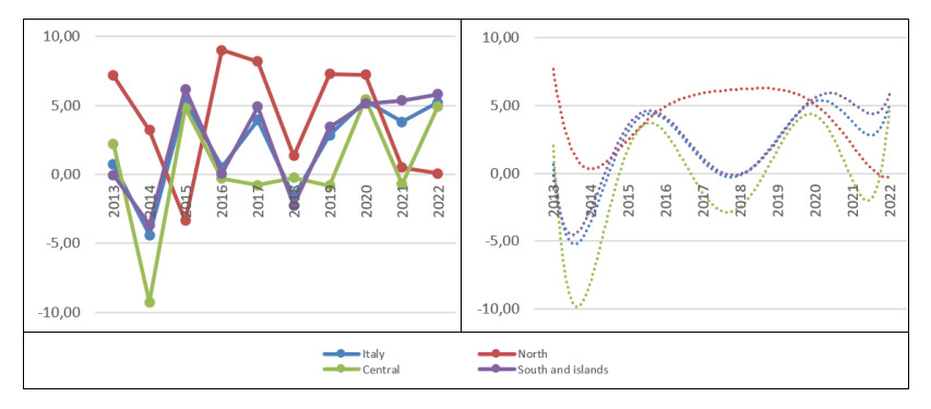
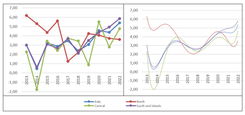
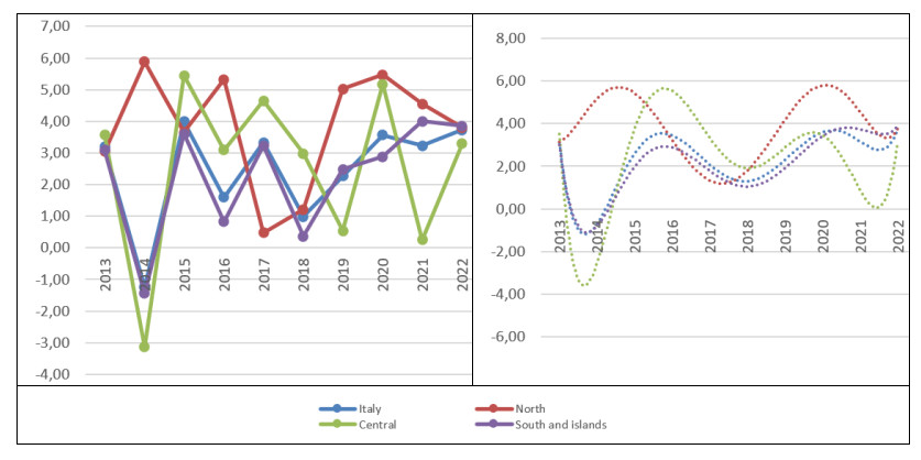
Italian olive oil companies play a significant role in this nation's economy, which is among the top in the world for its geomorphological and meteorological characteristics. This research analyzed the performance of three profitability ratios (return on equity (R.O.E.), return on investment (R.O.I.), and return on sales (R.O.S.)) of 3184 companies from 2013 to 2022. Average ratios for each year and critical descriptive statistics were calculated. Broken lines and interpolating curves, obtained from sixth-degree polynomial equations maximizing R2, represent the trends. One-way ANOVA and Tukey-Kramer methods facilitated statistical comparisons between macro-regions. Despite the regular consumption of olive oil, the profitability of businesses has been erratic and fluctuating, probably due to the varying productivity of raw material crops. The pandemic seems to have had no impact. There are no statistically significant differences between macro-areas. The results are helpful to Italian and foreign entrepreneurs who can relate their situation to the average situation in context, highlighting possible gaps that, if negative, must be bridged with a timely management review. National and supranational political authorities can also use this study to orient the frequent support policies in the agricultural and agro-industrial sectors. So too can the bodies in charge of food education, especially for young people, can encourage the use of olive oil where it is lacking. The main limitation of this study was its focus on a small set of profitability ratios. In the future, the study should consider other profitability and asset ratios and investigate investments in sustainability, keeping in mind that all enterprises should contribute to developing eco-friendly production systems.

| [1] | Accorsi R, Cascini A, Ferrari E, et al. (2013) Life cycle assessment of an extra-virgin olive oil supply chain, In Bevilacqua, M. (ed.) Proceeding of the XVⅡ Summer School Francesco Turco: A challenge for the future - The role of industrial engineering in a global sustainable economy, Senigallia (Ancona) Italy, September 11–13, 2013,172–178. https://hdl.handle.net/11585/197332 |
| [2] | Adamo P, Baldoni L, Benalia S, et al. (2020) Intensificazione sostenibile. Proceedings of the 17th Conference A.I.S.S.A., February 2020, 1: 17–18. |
| [3] | Alfei B, Pannelli G, Ricci A (2013) Olivicoltura. Coltivazione, olio e territorio, Bologna, Edagricole. |
| [4] | Aparicio R, Harwood J (2013) Handbook of Olive Oil: Analysis and Properties, New York: Springer-Verlag NY Inc. https://doi.org/10.1007/978-1-4614-7777-8 |
| [5] | Attorre A, Ricci N, Soracco D (2021) Il mondo dell'olio. Storia, produzione, uso in cucina dell'extravergine, Bra: Slow Food. |
| [6] | Benedetti M, Corti F, Guagnini C (Yearless) Agroalimentare: Italia, una (pen)isola felice, Available from: https://www.sace.it/docs/default-source/default-document-library/sace-focus-on-agroalimentare.pdf?sfvrsn = 87a146b9_0 (accessed on 4 July 2024) |
| [7] |
Bhattacharya S, Momaya KS, Iyer KC (2020) Benchmarking enablers to achieve growth performance: a conceptual framework. Benchmarking 27: 1475–1501. https://doi.org/10.1108/BIJ-08-2019-0376 doi: 10.1108/BIJ-08-2019-0376

|
| [8] |
Boesen S, Bey N, Niero M (2019) Environmental sustainability of liquid food packaging: Is there a gap between Danish consumers' perception and learnings from life cycle assessment? J Clean Prod 210: 1193–1206. https://doi.org/10.1016/j.jclepro.2018.11.055 doi: 10.1016/j.jclepro.2018.11.055
|
| [9] | Boria P (2023) L'evasione fiscale. Ricerca su natura giuridica e dimensione quantitativa, Roma: Università La Sapienza. |
| [10] | Borsellino V, Zinnanti C, Migliore G, et al. (2018) An exploratory analysis of website quality in the agrifood sector: The case of extra virgin olive oil. Quality - Access to Success 19: 132–138. |
| [11] | Boskou D (2006) Olive Oil. Chemistry and Technology, New York: A.O.C.S. https://doi.org/10.4324/9781003040217 |
| [12] | Boskou D (2015) Olive and Olive Oil Bioactive Constituents, New York: A.O.C.S. https://doi.org/10.1016/B978-1-63067-041-2.50007-0 |
| [13] | Caricato L (2017) OOF International Magazine. The shapes of oil. Packaging, the silent revolution, Milano: Olio Officina. |
| [14] |
Castilla-Polo F, Gallardo-Vázquez D, Sánchez-Hernández MI, et al. (2018) An empirical approach to analyze the reputation-performance linkage in agrifood cooperatives. J Clean Prod 195: 163–175. https://doi.org/10.1016/j.jclepro.2018.05.210 doi: 10.1016/j.jclepro.2018.05.210
|
| [15] | Conte L, Servili M (2022) Oleum. Qualità, tecnologia e sostenibilità degli oli da olive, Bologna: Edagricole. |
| [16] | Contò F (2005) Economia e organizzazione delle filiere agroalimentari. La filiera dell'olio di oliva di qualità, Milano: Franco Angeli. |
| [17] |
De Blasio V, Pavone P, Migliaccio G (2022) Cosmetics companies: income developments in time of crisis. J Small Bus Enterp D 29: 1017–1048. https://doi.org/10.1108/JSBED-11-2019-0369 doi: 10.1108/JSBED-11-2019-0369
|
| [18] |
De Gennaro B, Notarnicola B, Roselli L, et al. (2012) Innovative olive-growing models: An environmental and economic assessment. J Clean Prod 28: 70–80. https://doi.org/10.1016/j.jclepro.2011.11.004 doi: 10.1016/j.jclepro.2011.11.004
|
| [19] | Di Gioia F (2022) Olivicoltura e produzione dell'olio di oliva, Roma: Andromeda. |
| [20] | Di Schino J, Liguori G, Stefani M (2016) L' oro del Mediterraneo. Olio d'oliva, Firenze: goWare. |
| [21] | Felice E (2007) Divari regionali e intervento pubblico. Per una rilettura dello sviluppo in Italia, Bologna: Il Mulino. |
| [22] | Fink A (1995) How to AnalyzeSurvey Data, Los Angeles: U.C.L.A. |
| [23] |
Fusco F, Migliaccio G (2018) Crisis, Sectoral and Geographical Factors: Financial Dynamics of Italian Cooperatives. Euromed J Bus 13: 130–148. https://doi.org/10.1108/EMJB-02-2016-0002 doi: 10.1108/EMJB-02-2016-0002
|
| [24] |
Fusco F, Migliaccio G (2019) Cooperatives and Crisis: Economic Dynamics in Italian Context. Int J Bus Glob 22: 638–654. https://doi.org/10.1504/IJBG.2019.100258 doi: 10.1504/IJBG.2019.100258
|
| [25] | Garibaldi R (2024) Turismo dell'olio. Available from: https://www.robertagaribaldi.it. |
| [26] |
Gómez-Carmona D, Paramio A, Cruces-Montes S, et al. (2023) The effect of the wine tourism experience. J Destin Mark Manage 29: 100793. https://doi.org/10.1016/j.jdmm.2023.100793 doi: 10.1016/j.jdmm.2023.100793
|
| [27] | Gorgitano MT, Sodano V (2019) Differentiation policies in the Italian market of extra virgin olive oil. Quality - Access to Success 20: 274–279. |
| [28] | Gu C (2013) Smoothing Spline ANOVA Models. 2nd ed., New York: Springer. https://doi.org/10.1007/978-1-4614-5369-7 |
| [29] | Gurrieri AR, Spallini S (2016) Networking Entrepreneurship in Non-Technology Sectors. The Case of Olive Oil, Developments in Marketing Science: Proceedings of the Academy of Marketing Science, 343–346. https://doi.org/10.1007/978-3-319-29877-1_69 |
| [30] | Hernández-Mogollón JM, Di-Clemente E, Campón-Cerro AM, et al. (2021) Olive oil tourism in the euro-mediterranean area. Int J Euro-Mediterr Stud 14: 85–101. |
| [31] |
Iovino F, Migliaccio G (2019) Financial Dynamics of Energy Companies During Global Economic Crisis. Int J Bus Glob 22: 541–554. https://doi.org/10.1504/IJBG.2019.100256 doi: 10.1504/IJBG.2019.100256
|
| [32] | Ismea (2021) Olio di oliva - Ultime dal settore. Olio di oliva: le prime stime produttive in Italia. Available from: https://www.ismeamercati.it/flex/cm/pages/ServeBLOB.php/L/IT/IDPagina/11750 (accessed on 4 July 2024). |
| [33] | Kharlamova O, Tkachenko S, Poliakova Y, et al. (2020) Management accounting using benchmarking tools. Acade Account Financ Stud J 24: 1–7. |
| [34] |
Kramer CY (1956) Extension of multiple range tests to group means with unequal numbers of replications. Biometrics 12: 307–310. https://doi.org/10.2307/3001469 doi: 10.2307/3001469
|
| [35] | Lanzara O (2017) Quando la qualità si fa concorrenza: il made in Italy e la legge 'Salva olio'. Il diritto dell'agricoltura, 127–156. |
| [36] | Liao Q, Li J (2018) An Adaptive Reduced Basis ANOVA method for High-dimensional Bayesian Inverse Problems. J Comput Physics, arXiv: 1811.05151[math.NA]. https://doi.org/10.1016/j.jcp.2019.06.059 |
| [37] | Lupi R (2020) Manuale di evasione fiscale. Conoscerla per contrastarla. Roma: Castelvecchi. |
| [38] | Mella P, Navaroni M (2016) Analisi di bilancio, Sant'Arcangelo di Romagna: Maggioli. |
| [39] | Menzani T (2007) Prima e dopo Mezzogiorno. Le regioni italiane fra arretratezza e sviluppo, Meridiana - Rivista di storia e scienze sociali (58-Nuove forme di democrazia), 245–249. |
| [40] |
Mesic Ž, Molnár A, Cerjak M (2018) Assessment of traditional food supply chain performance using triadic approach: the role of relationships quality. Supply Chain Manage 23: 396–411. https://doi.org/10.1108/SCM-10-2017-0336 doi: 10.1108/SCM-10-2017-0336
|
| [41] | Migliaccio G (2018) The profitability of Italian hotels during and after the 2008 Economic Crisis. Afr J Hosp Tour Leisure 7: 1–21. |
| [42] |
Migliaccio G, Arena MF (2021a) Il benchmarking per il controllo della performance: esiti di una ricerca nei distretti conciari italiani. Manage Control, 87–110. https://doi.org/10.3280/MACO2021-003005 doi: 10.3280/MACO2021-003005
|
| [43] |
Migliaccio G, Arena MF (2021b) Financial performance of Italian tanning manufacturers before, during and after the global crisis. Int J Glob Small Bus 12: 213–246. https://doi.org/10.1504/IJGSB.2021.10040807 doi: 10.1504/IJGSB.2021.10040807
|
| [44] |
Migliaccio G, D'Alelio CC (2022) The profitability of Italian jewellery between the two international economic crisis. Int J Glob Small Bus 13: 79–107. https://doi.org/10.1504/IJGSB.2022.10047040 doi: 10.1504/IJGSB.2022.10047040
|
| [45] |
Migliaccio G, De Blasio V (2024) The Italian Plastics Industries toward a Plastic-Free Society: what Possible Strategies? World Rev Entrep Manage Sust Dev 20: 179–218. https://doi.org/10.1504/WREMSD.2024.10061683 doi: 10.1504/WREMSD.2024.10061683
|
| [46] |
Migliaccio G, De Palma A (2024) Profitability and financial performance of Italian real estate companies: quantitative profiles. Int J Product Perfor Manage 73: 122–160. https://doi.org/10.1108/IJPPM-02-2023-0075 doi: 10.1108/IJPPM-02-2023-0075
|
| [47] |
Migliaccio G, Lucadamo A, Napoli G, et al. (2022) Economic and Sporting Performance and Player Registration Rights in Italian Soccer: Connections? Int J Manage Enterp Dev 21: 392–415. https://doi.org/10.1504/IJMED.2022.126577 doi: 10.1504/IJMED.2022.126577
|
| [48] |
Migliaccio G, Pavone P (2021a) Innovative Small Start-Ups in Italy: a Successful Business Model? Int J Manage Enterp Dev 20: 405–455. https://doi.org/10.1504/IJMED.2022.10042082 doi: 10.1504/IJMED.2022.10042082
|
| [49] | Migliaccio G, Pavone P (2021b) Italian Innovative Start-up Cohorts: an Empirical Survey on Profitability, in Bevilacqua, C., Calabrò, F. and Della Spina, L. (Eds.), New Metropolitan Perspectives - Knowledge Dynamics and Innovation-driven Policies Towards Urban and Regional Transition (Vol. 2), Springer Nature Switzerland AG, Heidelberg & Berlin, 834–843. https://doi.org/10.1007/978-3-030-48279-4 |
| [50] |
Migliaccio G, Pavone P (2022) Primary sector in Italy: profitability dynamics and relationship with the international economic crisis. Int J Product Perfor Manage 71: 2893–2912. https://doi/10.1108/IJPPM-05-2020-0229 doi: 10.1108/IJPPM-05-2020-0229
|
| [51] |
Migliaccio G, Pavone P (2024) Innovativeness in the economic system: the Italian experience. Int J Bus Innov Res 34: 109–138. https://doi.org/10.1504/IJBIR.2024.138141 doi: 10.1504/IJBIR.2024.138141
|
| [52] |
Migliaccio G, Tucci L (2020) Economic assets and financial performance of Italian wine companies. Int J Wine Bus Res 32: 325–352. https://doi.org/10.1108/IJWBR-04-2019-0026 doi: 10.1108/IJWBR-04-2019-0026
|
| [53] | Migliaccio G, Tucci L, Simonetti B (2021) The Effects of the Global Crisis on the Economic-Financial Performance of Italian Bed and Breakfasts: a Ten-year Quantitative Analysis from the Financial reports. e-Rev Tour Res 18: 611–646. |
| [54] | Moro E (2014) La dieta mediterranea. Mito e storia di uno stile di vita, Bologna: Il Mulino. |
| [55] | Pato ML (2024) A Decade of Olive Oil Tourism: A Bibliometric Survey. Sustainability (Switzerland), 16: 1665. https://doi.org/10.3390/su16041665 |
| [56] |
Pavone P, Migliaccio G (2021) Profitability of the Italian farming companies and the impact of financial crisis: quantitative research using accounting data. Int J Bus Perfor Manage 22: 394–425. https://doi.org/10.1504/IJBPM.2021.10041320 doi: 10.1504/IJBPM.2021.10041320
|
| [57] |
Pavone P, Migliaccio G, Simonetti B (2023) Investigating financial statements in hospitality: a quantitative approach. Qual Quant 57: S383–S407. https://doi.org/10.1007/s11135-020-01086-3 doi: 10.1007/s11135-020-01086-3
|
| [58] |
Pellegrini G, La Sala P, Camposeo S et al. (2017) Economic sustainability of the olive oil high and super-high density cropping systems in Italy. Global Bus Econ Rev 19: 553–569. https://doi.org/10.1504/GBER.2017.086604 doi: 10.1504/GBER.2017.086604
|
| [59] | Preedy VR, Watson RR (2020) Olives and Olive Oil in Health and Disease Prevention, Amsterdam: Elsevier. |
| [60] |
Pulido-Fernández JI, Casado-Montilla J, Carrillo-Hidalgo I, et al. (2022) Evaluating olive oil tourism experiences based on the segmentation of demand. Int J Gastron Food Sci 27: 100461. https://doi.org/10.1016/j.ijgfs.2021.100461 doi: 10.1016/j.ijgfs.2021.100461
|
| [61] | Ross A, Willson VL (2017) One-way ANOVA. In Ross, A., Willson V.L. (Eds.), Basic and Advanced Statistical Tests. Sense: Rotterdam, 21–24. https://doi.org/10.1007/978-94-6351-086-8_5 |
| [62] | Rossi R (2017) Il settore delle olive e dell'olio d'oliva nell'UE. Principali caratteristiche, sfide e prospettive. Available from: https://www.europarl.europa.eu/RegData/etudes/BRIE/2017/608690/EPRS_BRI%282017%29608690_IT.pdf (accessed on 4 July 2024). |
| [63] |
Sanchez-Famoso V, Cano-Rubio M, Fuentes-Lombardo G (2019) The role of cooperation agreements in the internationalization of Spanish winery and olive oil family firms. Int J Wine Bus Res 31: 555–577. https://doi.org/10.1108/IJWBR-08-2018-0042 doi: 10.1108/IJWBR-08-2018-0042
|
| [64] | Sarnari T (2022) Tendenze e dinamiche recenti. Olio d'oliva. Available from: https://olivonews.it/wp-content/uploads/2022/09/20221309_Tendenze_olio.pdf. |
| [65] | Scarfì P (2024) Evasione fiscale. Un'idea che risolve la questione. Tricase: Youcanprint. |
| [66] | Scarpato D, Borrelli IP, Ardeleanu MP (2013) Competitiveness and environmental performance in the olive oil sector: An analysis of the Campania region. Qual - Access Success 14: 165–169. |
| [67] |
Scherhag K, Rüdiger J, Dreyer A (2023) Introduction to wine tourism. Zeitschrift für Tourismuswissenschaft 15: 231–238. https://doi.org/10.2307/3001913 doi: 10.2307/3001913
|
| [68] | Solari A, Salmaso L, Pesarin F, et al. (2009) Permutation Tests for Stochastic Ordering and ANOVA. Theory and Applications with R., 194. New York: Springer-Verlag. http://dx.doi.org/10.1007/978-0-387-85956-9 |
| [69] | Soós G, Dávid L (2015) Wine Marketing - Tools for Innovation, Creativity and Sustainability, Proceedings of International Conference on New Trends in Sustainable Business and Consumption (B.A.S.I.Q. 2015), Bucharest, JUN 18-19, 2015,473–480. |
| [70] | Stillitano T, De Luca AI, Iofrida N, et al. (2017) Economic analysis of olive oil production systems in southern Italy. Qual - Access Success 18: 107–112. |
| [71] |
Tukey JW (1949) Comparing individual means in the analysis of variance. Biometrics 5: 99–114. https://doi.org/10.2307/3001913 doi: 10.2307/3001913
|
| [72] | Tukey JW (1953) The problem of multiple comparisons. unpublished manuscript, In: Karen, The Collected Works of John W Tukey VIII. Multiple Comparisons: 1948–1983. New York: Chapman and Hall. |
| [73] | Tukey JW (1993) Where should multiple comparisons go next? In: Hoppe, F.M., Multiple Comparisons, Selection, and Applications in Biometry. New York: Dekkerpp, 187–207. |
| [74] |
Vena-Oya J, Parrilla-González JA (2023) Importance–performance analysis of olive oil tourism activities: Differences between national and international tourists. J Vacat Market. https://doi.org/10.1177/13567667221147316 doi: 10.1177/13567667221147316
|
| [75] | Viesti G (2021) Centri e periferie. Europa, Italia, Mezzogiorno dal XX al XXI secolo, Bari-Roma: La Terza. |
| [76] | Watson GH (2000) Il Benchmarking. Come Migliorare i Processi e la Competitività Aziendale Adattando e Adottando le Pratiche Delle Imprese Leader, Milano: Franco Angeli. |
Figures(7) / Tables(18)

Guido Migliaccio, Antonella De Blasio. The economic performance of Italian olive oil companies: a comparative quantitative approach using the Anova and Tukey-Kramer methods[J]. Quantitative Finance and Economics, 2024, 8(3): 437-465. doi: 10.3934/QFE.2024017


 DownLoad: