The cyclic AMP response element–binding protein (CREB) and nerve growth factor (NGF) have been proposed as key modulators of brain health and are involved in synaptic plasticity. The study investigates how combined water-based training affects hippocampal neuron plasticity and memory function in old rats.
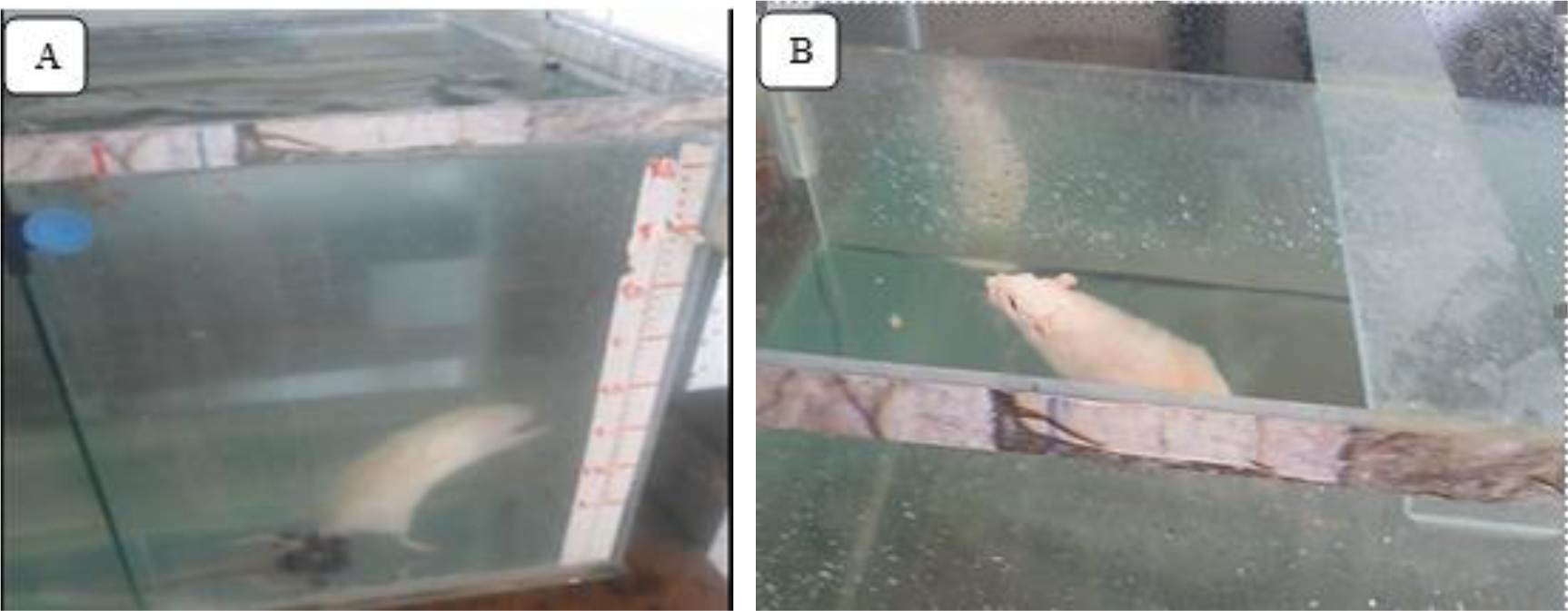
16 Wistar male rats 24-month-old were randomly divided into two groups: combined training (n = 8) and control (n = 8). Four sessions were performed per week for 10 weeks, and consisted of resistance and endurance training in water. The control group was placed in a water container during training for 30 minutes to be homogenized in terms of the stress conditions. The.NGF and CREB genes in the hippocampus were evaluated and the working memory was measured using real-time PCR and Y-maze tests. The SPSS 26 software was utilized in which independent t-tests were used to analyze the genes and the Mann-Whitney U test was used to analyze functional memory with a significant level of (P < 0.05).
The combined training resulted in a significant rise in NGF and CREB gene expression in the hippocampus tissue of elderly rats compared to the control group (P < 0.05); however, there was no notable difference in the Y maze performance test between the two groups (P < 0.05).
These findings suggest that water-based combined training has beneficial effects on gene expression of NGF and CREB; however, it is necessary to conduct more studies to comprehend the effects of combined training on memory function.
Citation: Roya. Askari, Mohadeseh. NasrAbadi, Amir Hossein. Haghighi, Mohammad Jahan Mahin, Rajabi Somayeh, Matteo. Pusceddu. Effect of combined training in water on hippocampal neuronal Plasticity and memory function in healthy elderly rats[J]. AIMS Neuroscience, 2024, 11(3): 260-274. doi: 10.3934/Neuroscience.2024017
The cyclic AMP response element–binding protein (CREB) and nerve growth factor (NGF) have been proposed as key modulators of brain health and are involved in synaptic plasticity. The study investigates how combined water-based training affects hippocampal neuron plasticity and memory function in old rats.
16 Wistar male rats 24-month-old were randomly divided into two groups: combined training (n = 8) and control (n = 8). Four sessions were performed per week for 10 weeks, and consisted of resistance and endurance training in water. The control group was placed in a water container during training for 30 minutes to be homogenized in terms of the stress conditions. The.NGF and CREB genes in the hippocampus were evaluated and the working memory was measured using real-time PCR and Y-maze tests. The SPSS 26 software was utilized in which independent t-tests were used to analyze the genes and the Mann-Whitney U test was used to analyze functional memory with a significant level of (P < 0.05).
The combined training resulted in a significant rise in NGF and CREB gene expression in the hippocampus tissue of elderly rats compared to the control group (P < 0.05); however, there was no notable difference in the Y maze performance test between the two groups (P < 0.05).
These findings suggest that water-based combined training has beneficial effects on gene expression of NGF and CREB; however, it is necessary to conduct more studies to comprehend the effects of combined training on memory function.

| [1] |
Pac A, Tobiasz-Adamczyk B, Błędowski P, et al. (2019) Influence of sociodemographic, behavioral and other health-related factors on healthy ageing based on three operative definitions. J Nutr Health Aging 23: 862-869. https://doi.org/10.1007/s12603-019-1243-5 
|
| [2] | Amarya S, Singh K, Sabharwal M (2018) Ageing process and physiological changes. Gerontology . Intech. https://doi.org/10.5772/intechopen.76249 |
| [3] |
Lu W, Pikhart H, Sacker A (2019) Domains and measurements of healthy aging in epidemiological studies: a review. Gerontologist 59: e294-e310. https://doi.org/10.1093/geront/gny029
|
| [4] |
Huang T, Larsen K, Ried-Larsen M, et al. (2014) The effects of physical activity and exercise on brain-derived neurotrophic factor in healthy humans: A review. Scand J Med Sci Sports 24: 1-10. https://doi.org/10.1111/sms.12069
|
| [5] |
Bonanni R, Cariati I, Tarantino U, et al. (2022) Physical exercise and health: a focus on its protective role in neurodegenerative diseases. J Funct Morphol Kinesiol 7: 38. https://doi.org/10.3390/jfmk7020038
|
| [6] |
Tomlinson L, Leiton CV, Colognato H (2016) Behavioral experiences as drivers of oligodendrocyte lineage dynamics and myelin plasticity. Neuropharmacology 110: 548-562. https://doi.org/10.1016/j.neuropharm.2015.09.016
|
| [7] |
Varela RB, Valvassori SS, Lopes-Borges J, et al. (2015) Sodium butyrate and mood stabilizers block ouabain-induced hyperlocomotion and increase BDNF, NGF and GDNF levels in brain of Wistar rats. J Psychiatr Res 61: 114-121. https://doi.org/10.1016/j.jpsychires.2014.11.003
|
| [8] |
Budni J, Bellettini-Santos T, Mina F, et al. (2015) The involvement of BDNF, NGF and GDNF in aging and Alzheimer's disease. Aging Dis 6: 331. https://doi.org/10.14336/AD.2015.0825
|
| [9] |
Murawska-Ciałowicz E, Wiatr M, Ciałowicz M, et al. (2021) BDNF impact on biological markers of depression—role of physical exercise and training. Int J Env Res Pub He 18: 7553. https://doi.org/10.3390/ijerph18147553
|
| [10] | Mitra S, Behbahani H, Eriksdotter M (2019) Innovative therapy for Alzheimer's disease-with focus on biodelivery of NGF. Front Neurosci 13. https://doi.org/10.3389/fnins.2019.00038 |
| [11] |
Allard S, Jacobs ML, Do Carmo S, et al. (2018) Compromise of cortical proNGF maturation causes selective retrograde atrophy in cholinergic nucleus basalis neurons. Neurobiol Aging 67: 10-20. https://doi.org/10.1016/j.neurobiolaging.2018.03.002
|
| [12] |
Chae C-H, Kim H-T (2009) Forced, moderate-intensity treadmill exercise suppresses apoptosis by increasing the level of NGF and stimulating phosphatidylinositol 3-kinase signaling in the hippocampus of induced aging rats. Neurochem Int 55: 208-213. https://doi.org/10.1016/j.neuint.2009.02.024
|
| [13] |
Dehbozorgi A, Tabrizi LB, Hosseini SA, et al. (2020) Effects of Swimming Training and Royal Jelly on BDNF and NGF Gene Expression in Hippocampus Tissue of Rats with Alzheimer's Disease. Zahedan J Res Med Sci 22: e98310. https://doi.org/10.5812/zjrms.98310
|
| [14] |
Hong Y-P, Lee H-C, Kim H-T (2015) Treadmill exercise after social isolation increases the levels of NGF, BDNF, and synapsin I to induce survival of neurons in the hippocampus, and improves depression-like behavior. J Exer Nutr Biochem 19: 11. https://doi.org/10.5717/jenb.2015.19.1.11
|
| [15] |
Kandel ER (2012) The molecular biology of memory: cAMP, PKA, CRE, CREB-1, CREB-2, and CPEB. Mol Brain 5: 1-12. https://doi.org/10.1186/1756-6606-5-14
|
| [16] |
Matos MR, Visser E, Kramvis I, et al. (2019) Memory strength gates the involvement of a CREB-dependent cortical fear engram in remote memory. Nat Commun 10: 2315. https://doi.org/10.1038/s41467-019-10266-1
|
| [17] |
Aguiar AS, Castro AA, Moreira EL, et al. (2011) Short bouts of mild-intensity physical exercise improve spatial learning and memory in aging rats: involvement of hippocampal plasticity via AKT, CREB and BDNF signaling. Mech Ageing Dev 132: 560-567. https://doi.org/10.1016/j.mad.2011.09.005
|
| [18] |
Li X, Wang L, Zhang S, et al. (2019) Timing-dependent protection of swimming exercise against d-galactose-induced aging-like impairments in spatial learning/memory in rats. Brain Sci 9: 236. https://doi.org/10.3390/brainsci9090236
|
| [19] |
Sabouri M, Kordi M, Shabkhiz F, et al. (2020) Moderate treadmill exercise improves spatial learning and memory deficits possibly via changing PDE-5, IL-1 β and pCREB expression. Exp Gerontol 139: 111056. https://doi.org/10.1016/j.exger.2020.111056
|
| [20] | Tunca U, Saygin M, Ozmen O, et al. (2021) The impact of moderate-intensity swimming exercise on learning and memory in aged rats: The role of Sirtuin-1. Iran J Basic Med Sci 24: 1413. |
| [21] |
Vilela TC, Muller AP, Damiani AP, et al. (2017) Strength and aerobic exercises improve spatial memory in aging rats through stimulating distinct neuroplasticity mechanisms. Mol Neurobiol 54: 7928-7937. https://doi.org/10.1007/s12035-016-0272-x
|
| [22] |
Yoo J-H (2020) The psychological effects of water-based exercise in older adults: an integrative review. Geriatr Nurs 41: 717-723. https://doi.org/10.1016/j.gerinurse.2020.04.019
|
| [23] |
Fedor A, Garcia S, Gunstad J (2015) The effects of a brief, water-based exercise intervention on cognitive function in older adults. Arch Clin Neuropsych 30: 139-147. https://doi.org/10.1093/arclin/acv001
|
| [24] | Jahanmahin M, Askari R, Haghighi A, et al. (2022) The Effect of 10 Weeks Combined Training in Water on Immunosenescence in Elderly Rats. J Isfahan Med School 40: 890-899. |
| [25] | Bryczkowska I, Baranowska-Bosiacka I, Lubkowska A (2017) Effect of repeated cold water swimming exercise on adaptive changes in body weight in older rats. Central Eur J Sport Sci Med 18: 77-87. https://doi.org/10.18276/cej.2017.2-08 |
| [26] |
Silva RTB, Castro PVd, Coutinho MPG, et al. (2017) Resistance jump training may reverse the weakened biomechanical behavior of tendons of diabetic Wistar rats. Fisioterapia e Pesquisa 24: 399-405. https://doi.org/10.1590/1809-2950/17198024042017
|
| [27] |
Xie Y, Li Z, Wang Y, et al. (2019) Effects of moderate-versus high-intensity swimming training on inflammatory and CD4+ T cell subset profiles in experimental autoimmune encephalomyelitis mice. J Neuroimmunol 328: 60-67. https://doi.org/10.1016/j.jneuroim.2018.12.005
|
| [28] | Altarifi AA, Kalha Z, Kana'An SF, et al. (2019) Effects of combined swimming exercise and non‑steroidal anti‑inflammatory drugs on inflammatory nociception in rats. Exp Ther Med 17: 4303-4311. https://doi.org/10.3892/etm.2019.7413 |
| [29] |
Shi X, Bai H, Wang J, et al. (2021) Behavioral assessment of sensory, motor, emotion, and cognition in rodent models of intracerebral hemorrhage. Front Neurol 12: 667511. https://doi.org/10.3389/fneur.2021.667511
|
| [30] |
Babaei P, Azari HB (2022) Exercise training improves memory performance in older adults: a narrative review of evidence and possible mechanisms. Front Hum Neurosci 15: 771553. https://doi.org/10.3389/fnhum.2021.771553
|
| [31] |
Lin J-Y, Kuo W-W, Baskaran R, et al. (2020) Swimming exercise stimulates IGF1/PI3K/Akt and AMPK/SIRT1/PGC1α survival signaling to suppress apoptosis and inflammation in aging hippocampus. Aging (Albany NY) 12: 6852. https://doi.org/10.18632/aging.103046
|
| [32] |
Naletova I, Satriano C, Pietropaolo A, et al. (2019) The copper (II)-assisted connection between NGF and BDNF by means of nerve growth factor-mimicking short peptides. Cells 8: 301. https://doi.org/10.3390/cells8040301
|
| [33] |
Niewiadomska G, Mietelska-Porowska A, Mazurkiewicz M (2011) The cholinergic system, nerve growth factor and the cytoskeleton. Behav Brain Res 221: 515-526. https://doi.org/10.1016/j.bbr.2010.02.024
|
| [34] |
Aguiar A, Boemer G, Rial D, et al. (2010) High-intensity physical exercise disrupts implicit memory in mice: involvement of the striatal glutathione antioxidant system and intracellular signaling. Neuroscience 171: 1216-1227. https://doi.org/10.1016/j.neuroscience.2010.09.053
|
| [35] |
Mohseni I, Peeri M, Azarbayjani MA (2020) Dietary supplementation with Salvia officinalis L. and aerobic training attenuates memory deficits via the CREB-BDNF pathway in amyloid beta-injected rats. J Med Plants 1: 119-132. https://doi.org/10.29252/jmp.1.73.119
|
| [36] |
Aoki C, Wu K, Elste A, et al. (2000) Localization of brain-derived neurotrophic factor and TrkB receptors to postsynaptic densities of adult rat cerebral cortex. J Neurosci Res 59: 454-463. https://doi.org/10.1002/(SICI)1097-4547(20000201)59:3<454::AID-JNR21>3.0.CO;2-H
|
| [37] |
Vaynman S, Ying Z, Gomez-Pinilla F (2003) Interplay between brain-derived neurotrophic factor and signal transduction modulators in the regulation of the effects of exercise on synaptic-plasticity. Neuroscience 122: 647-657. https://doi.org/10.1016/j.neuroscience.2003.08.001
|
| [38] |
Cechella JL, Leite MR, Rosario AR, et al. (2014) Diphenyl diselenide-supplemented diet and swimming exercise enhance novel object recognition memory in old rats. Age 36: 1-10. https://doi.org/10.1007/s11357-014-9666-8
|
| [39] |
Jin Y, Li X, Wei C, et al. (2024) Effects of exercise-targeted hippocampal PDE-4 methylation on synaptic plasticity and spatial learning/memory impairments in D-galactose-induced aging rats. Exp Brain Res 242: 309-320. https://doi.org/10.1007/s00221-023-06749-9
|
| [40] |
Feter N, Penny J, Freitas M, et al. (2018) Effect of physical exercise on hippocampal volume in adults: Systematic review and meta-analysis. Sci Sport 33: 327-338. https://doi.org/10.1016/j.scispo.2018.02.011
|
| [41] |
Vints WA, Šeikinaitė J, Gökçe E, et al. (2024) Resistance exercise effects on hippocampus subfield volumes and biomarkers of neuroplasticity and neuroinflammation in older adults with low and high risk of mild cognitive impairment: a randomized controlled trial. GeroScience 46: 3971-3991. https://doi.org/10.1007/s11357-024-01110-6
|
| [42] |
Zimmerman B, Rypma B, Gratton G, et al. (2021) Age-related changes in cerebrovascular health and their effects on neural function and cognition: A comprehensive review. Psychophysiology 58: e13796. https://doi.org/10.1111/psyp.13796
|
| [43] |
Corbi G, Conti V, Filippelli A, et al. (2015) The role of physical activity on the prevention of cognitive impairment. Translational medicine@ UniSa 13: 42.
|
| [44] | Vints WA, Levin O, Fujiyama H, et al. (2022) Exerkines and long-term synaptic potentiation: Mechanisms of exercise-induced neuroplasticity. Front Neuroendocrin 66: 1-27. https://doi.org/10.1016/j.yfrne.2022.100993 |
| [45] | Di Raimondo D, Rizzo G, Musiari G, et al. (2020) Role of regular physical activity in neuroprotection against acute ischemia. Int J Mol Sci 21: 1-30. https://doi.org/10.3390/ijms21239086 |
| [46] |
Damirchi A, Tehrani BS, Alamdari KA, et al. (2014) Influence of aerobic training and detraining on serum BDNF, insulin resistance, and metabolic risk factors in middle-aged men diagnosed with metabolic syndrome. Clin J Sport Med 24: 513-518. https://doi.org/10.1097/JSM.0000000000000082
|
| [47] |
Kelly ME, Duff H, Kelly S, et al. (2017) The impact of social activities, social networks, social support and social relationships on the cognitive functioning of healthy older adults: a systematic review. Sys Rev 6: 1-18. https://doi.org/10.1186/s13643-017-0632-2
|
| [48] |
Sun Ln, Li Xl, Wang F, et al. (2017) High-intensity treadmill running impairs cognitive behavior and hippocampal synaptic plasticity of rats via activation of inflammatory response. J Neurosci Res 95: 1611-1620. https://doi.org/10.1002/jnr.23996
|
| [49] |
Baddeley A (2003) Working memory: looking back and looking forward. Nat Rev Neurosci 4: 829-839. https://doi.org/10.1038/nrn1201
|
| [50] |
Gothe N, Pontifex MB, Hillman C, et al. (2013) The acute effects of yoga on executive function. J Phys Act Health 10: 488-495. https://doi.org/10.1123/jpah.10.4.488
|
| [51] |
Kramer AF, Hahn S, Cohen NJ, et al. (1999) Ageing, fitness and neurocognitive function. Nature 400: 418-419. https://doi.org/10.1038/22682
|
| [52] |
Zhidong C, Wang X, Yin J, et al. (2021) Effects of physical exercise on working memory in older adults: a systematic and meta-analytic review. Eur Rev Aging Phys A 18: 1-15. https://doi.org/10.1186/s11556-021-00272-y
|


Figures(4) / Tables(3)

Roya. Askari, Mohadeseh. NasrAbadi, Amir Hossein. Haghighi, Mohammad Jahan Mahin, Rajabi Somayeh, Matteo. Pusceddu. Effect of combined training in water on hippocampal neuronal Plasticity and memory function in healthy elderly rats[J]. AIMS Neuroscience, 2024, 11(3): 260-274. doi: 10.3934/Neuroscience.2024017


 DownLoad: