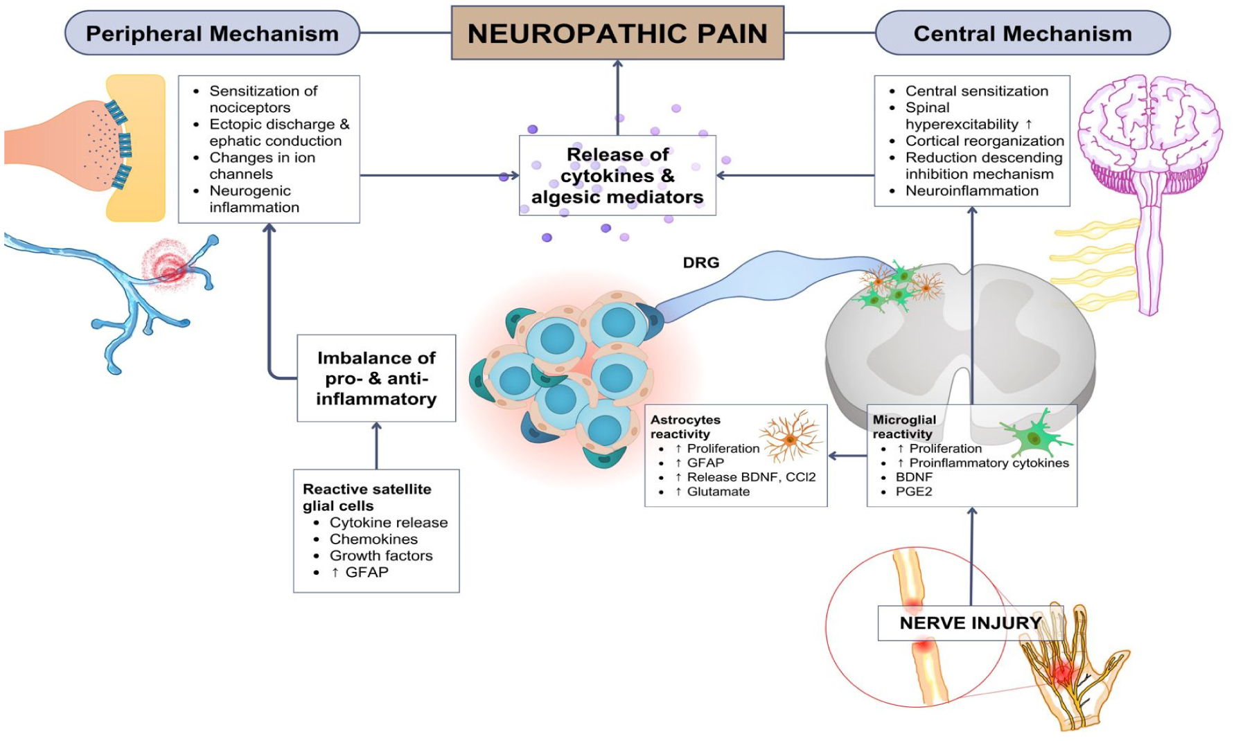
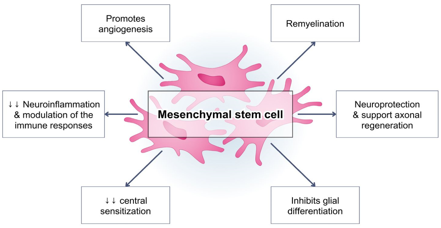
Pain is an essential aspect of the body's physiological response to unpleasant noxious stimuli from either external sustained injuries or an internal disease condition that occurs within the body. Generally, pain is temporary. However, in patients with neuropathic pain, the experienced pain is persistent and uncontrollable, with an unsatisfactory treatment effectiveness. The activation of the immune system is a crucial factor in both central and peripheral neuropathic pain. The immune response plays an important role in the progression of the stages of neuropathic pain, and acts not only as pain mediators, but also produce analgesic molecules. Neuropathic pain has long been described as a result of dysfunctional nerve activities. However, there is substantial evidence indicating that the regulation of hyperalgesia is mediated by astrocytes and microglia activation. Mesenchymal stem cells currently hold an optimal potential in managing pain, as they can migrate to damaged tissues and have a robust immunosuppressive role for autologous or heterologous transplantation. Moreover, mesenchymal stem cells revealed their immunomodulatory capabilities by secreting growth factors and cytokines through direct cell interactions. The main idea underlying the use of mesenchymal stem cells in pain management is that these cells can replace damaged nerve cells by releasing neurotrophic factors. This property makes them the perfect option to modulate and treat neuropathic pain, which is notoriously difficult to treat.
Citation: Ida Ayu Sri Wijayanti, I Made Oka Adnyana, I Putu Eka Widyadharma, I Gede Eka Wiratnaya, Tjokorda Gde Bagus Mahadewa, I Nyoman Mantik Astawa. Neuroinflammation mechanism underlying neuropathic pain: the role of mesenchymal stem cell in neuroglia[J]. AIMS Neuroscience, 2024, 11(3): 226-243. doi: 10.3934/Neuroscience.2024015
Pain is an essential aspect of the body's physiological response to unpleasant noxious stimuli from either external sustained injuries or an internal disease condition that occurs within the body. Generally, pain is temporary. However, in patients with neuropathic pain, the experienced pain is persistent and uncontrollable, with an unsatisfactory treatment effectiveness. The activation of the immune system is a crucial factor in both central and peripheral neuropathic pain. The immune response plays an important role in the progression of the stages of neuropathic pain, and acts not only as pain mediators, but also produce analgesic molecules. Neuropathic pain has long been described as a result of dysfunctional nerve activities. However, there is substantial evidence indicating that the regulation of hyperalgesia is mediated by astrocytes and microglia activation. Mesenchymal stem cells currently hold an optimal potential in managing pain, as they can migrate to damaged tissues and have a robust immunosuppressive role for autologous or heterologous transplantation. Moreover, mesenchymal stem cells revealed their immunomodulatory capabilities by secreting growth factors and cytokines through direct cell interactions. The main idea underlying the use of mesenchymal stem cells in pain management is that these cells can replace damaged nerve cells by releasing neurotrophic factors. This property makes them the perfect option to modulate and treat neuropathic pain, which is notoriously difficult to treat.

| [1] | Garcia-Larrea L (2014) The Pathophysiology of Neuropathic Pain: Critical Review of Models and Mechanisms Educational Objectives. Pain 2014 Refresher Courses: 15th World Congress on Pain : pp. 453-475. Available from: https://www.semanticscholar.org/paper/Pathophysiology-of-Neuropathic-Pain-%3A-Critical-of-GarciaLarrea/099cac98b142406cc3e25d51eda4a8c1b200e6ef#citing-papers |
| [2] | Miranda CCV, de Franco Seda Junior L, do Amaral Pelloso LRC (2016) New physiological classification of pains: current concept of neuropathic pain. Revista Dor 17: 3-5. https://doi.org/10.5935/1806-0013.20160037 |
| [3] |
Rosenberger DC, Blechschmidt V, Timmerman H, et al. (2020) Challenges of neuropathic pain: focus on diabetic neuropathy. J Neural Transm 127: 589-624. https://doi.org/10.1007/s00702-020-02145-7 
|
| [4] |
Joshi HP, Jo HJ, Kim YH, et al. (2021) Stem cell therapy for modulating neuroinflammation in neuropathic pain. Int J Mol Sci 22: 4853. https://doi.org/10.3390/ijms22094853
|
| [5] |
Kan H, Fan L, Gui X, et al. (2022) Stem cell therapy for neuropathic pain: A bibliometric and visual analysis. J Pain Res 15: 1797-1811. https://doi.org/10.2147/JPR.S365524
|
| [6] |
Huh Y, Ji RR, Chen G (2017) Neuroinflammation, bone marrow stem cells, and chronic pain. Front Immunol 8: 1014. https://doi.org/10.3389/fimmu.2017.01014
|
| [7] |
Finnerup NB, Kuner R, Jensen TS (2021) Neuropathic pain: Frommechanisms to treatment. Physiol Rev 101: 259-301. https://doi.org/10.1152/physrev.00045.2019
|
| [8] | Zhu Q, Yan Y, Zhang D, et al. (2021) Effects of pulsed radiofrequency on nerve repair and expressions of GFAP and GDNF in rats with neuropathic pain. BioMed Res Int . https://doi.org/10.1155/2021/9916978 |
| [9] |
Triolo D, Dina G, Lorenzetti I, et al. (2006) Loss of glial fibrillary acidic protein (GFAP) impairs Schwann cell proliferation and delays nerve regeneration after damage. J Cell Sci 119: 3981-93. https://doi.org/10.1242/jcs.03168
|
| [10] |
Borzan J, Meyer RA (2009) Neuropathic pain. Encyclopedia Neurosci : 749-757. https://doi.org/10.1016/B978-008045046-9.01926-4
|
| [11] | Cohen SP, Mao J (2014) Neuropathic pain: Mechanisms and their clinical implications. BMJ (Online) 348: f7656. https://doi.org/10.1136/bmj.f7656 |
| [12] | Chang K-H, Ro LS (2005) Neuropathic pain: Mechanisms and treatments. Chang Gung Med J 28: 597-605. Available at: https://www.ncbi.nlm.nih.gov/pubmed/16323550 |
| [13] |
Latremoliere A, Woolf CJ (2009) Central Sensitization: A generator of pain hypersensitivity by central neural plasticity. J Pain 10: 895-926. https://doi.org/10.1016/j.jpain.2009.06.012
|
| [14] |
Pratik D, Padhan A, Mohapatra S (2018) Mechanisms of neuropathic pain. Int J Livestock Res 8: 50. https://doi.org/10.5455/ijlr.20171128040037
|
| [15] |
Mika J, Zychowska M, Popiolek-Barczyk K, et al. (2013) Importance of glial activation in neuropathic pain. Eur J Pharmacol 716: 106-119. https://doi.org/10.1016/j.ejphar.2013.01.072
|
| [16] |
Zhao H, Alam A, Chen Q, et al. (2017) The role of microglia in the pathobiology of neuropathic pain development: what do we know?. Br J Anaesth 118: 504-516. https://doi.org/10.1093/bja/aex006
|
| [17] |
Chen G, Zhang YQ, Qadri YJ, et al. (2018) Review microglia in pain: Detrimental and protective roles in pathogenesis and resolution of pain. Neuron 100: 1292-1311. https://doi.org/10.1016/j.neuron.2018.11.009
|
| [18] |
Baral P, Udit S, Chiu IM (2019) Pain and immunity: implications for host defence. Nat Rev Immunol 19: 433-447. https://doi.org/10.1038/s41577-019-0147-2
|
| [19] |
Gong L, Wu J, Zhou S, et al. (2016) Global analysis of transcriptome in dorsal root ganglia following peripheral nerve injury in rats. Biochem Biophys Res Commun 478: 206-12. http://dx.doi.org/10.1016/j.bbrc.2016.07.067
|
| [20] |
Montague K, Malcangio M (2017) The therapeutic potential of targeting chemokine signaling in the treatment of chronic pain. J Neurochem 141: 520-31. https://onlinelibrary.wiley.com/doi/abs/10.1111/jnc.13927
|
| [21] |
Li T, Chen X, Zhang C, et al. (2019) An update on reactive astrocytes in chronic pain. J Neuroinflammation 16: 1-13. https://doi.org/10.1186/s12974-019-1524-2
|
| [22] |
Ospelnikova TP, Shitova AD, Voskresenskaya ON, et al. (2023) Neuroinflammation in the pathogenesis of neuropathic pain syndrome. Neurosci Behav Physiol 53: 27-33. https://doi.org/10.1007/s11055-023-01387-8
|
| [23] | Schomberg D, Ahmed M, Miranpuri G, et al. (2012) Neuropathic pain: Role of inflammation, immune response, and ion channel activity in central injury mechanisms. Ann Neurosci 19: 125-132. https://doi.org/10.5214/ans.0972.7531.190309 |
| [24] |
Kotliarova A, Sidorova YA (2021) Glial cell line-derived neurotrophic factor family ligands, players at the interface of neuroinflammation and neuroprotection: Focus onto the glia. Front Cell Neurosci 15: 679034. https://doi.org/10.3389/fncel.2021.679034
|
| [25] | Widyadharma IPE (2021) The role of oxidative stress, inflammation and glial cell in pathophysiology of myofascial pain. Postepy Psychiatr Neurol 29: 180-6. https://doi.org/10.5114/ppn.2020.100036 |
| [26] |
Cairns BE, Arendt-nielsen L, Sacerdote P (2015) Perspectives in pain research 2014: Neuroinflammation and glial cell activation: The cause of transition from acute to chronic pain?. Scand J Pain 6: 3-6. https://doi.org/10.1016/j.sjpain.2014.10.002
|
| [27] | Lu HJ, Gao YJ (2022) Astrocytes in chronic pain: Cellular and molecular mechanisms. Neurosci Bull 39: 425-39. https://doi.org/10.1007/s12264-022-00961-3 |
| [28] |
Stevenson R, Samokhina E, Rossetti I, et al. (2020) Neuromodulation of glial function during neurodegeneration. Front Cell Neurosci 14: 1-23. https://doi.org/10.3389/fncel.2020.00278
|
| [29] |
Liddelow SA, Barres BA (2017) Reactive astrocytes: Production, function, and therapeutic potential. Immunity 46: 957-67. http://dx.doi.org/10.1016/j.immuni.2017.06.006
|
| [30] |
Yang Z, Wang KKW (2015) Glial fibrillary acidic protein: From intermediate filament assembly and gliosis to neurobiomarker. Trends Neurosci 38: 364-374. https://doi.org/10.1016/j.tins.2015.04.003
|
| [31] |
Tykhomyrov A, Pavlova AS, Nedzvetsky VS (2016) Glial fibrillary acidic protein (GFAP): on the 45th anniversary of its discovery. Neurophysiology 48: 54-71. https://doi.org/10.1007/s11062-016-9568-8
|
| [32] |
Frese L, Dijkman E, Hoerstrup SP (2016) Adipose Tissue-Derived Stem Cells in Regenerative. Transfus Med Hemother 43: 268-274. https://doi.org/10.1159/000448180
|
| [33] |
Vadivelu S, Willsey M, Curry DJ, et al. (2013) Potential role of stem cells for neuropathic pain disorders. Neurosurg Focus 35: 1-5. https://doi.org/10.3171/2013.6.FOCUS13235
|
| [34] |
Han YH, Kim KH, Abdi S, et al. (2019) Stem cell therapy in pain medicine. Korean J Pain 32: 245-55. https://doi.org/10.3344/kjp.2019.32.4.245
|
| [35] |
Ferrini F, Salio C, Boggio EM, et al. (2020) Interplay of BDNF and GDNF in the mature spinal somatosensory system and its potential therapeutic relevance. Curr Neuropharmacol 19: 1225-1245. https://doi.org/10.2174/1570159X18666201116143422
|
| [36] |
Chen G, Park CK, Xie RG, et al. (2015) Intrathecal bone marrow stromal cells inhibit neuropathic pain via TGF-β secretion. J Clin Invest 125: 3226-3240. https://doi.org/10.1172/JCI80883
|
| [37] |
Chiang CY, Liu SA, Sheu ML, et al. (2016) Feasibility of human amniotic fluid derived stem cells in alleviation of neuropathic pain in chronic constrictive injury nerve model. PLoS One 11. https://doi.org/10.1371/journal.pone.0159482
|
| [38] |
Mert T, Kurt AH, Altun İ, et al. (2017) Pulsed magnetic field enhances therapeutic efficiency of mesenchymal stem cells in chronic neuropathic pain model. Bioelectromagnetics 38: 255-64. https://doi.org/10.1002/bem.22038
|
| [39] | Xie J, Ren J, Liu N, et al. (2019) Pretreatment with AM1241 enhances the analgesic effect of intrathecally administrated mesenchymal stem cells. Stem Cells Int 2019: 7025473. https://doi.org/10.1155/2019/7025473 |
| [40] |
Al-Massri KF, Ahmed LA, El-Abhar HS (2019) Mesenchymal stem cells therapy enhances the efficacy of pregabalin and prevents its motor impairment in paclitaxel-induced neuropathy in rats: role of Notch1 receptor and JAK/STAT signaling pathway. Behav Brain Res 360: 303-11. https://doi.org/10.1016/j.bbr.2018.12.013
|
| [41] | Guo W, Chu YX, Imai S, et al. (2016) Further observations on the behavioral and neural effects of bone marrow stromal cells in rodent pain models. Molecular Pain 12: 1744806916658043. https://doi.org/10.1177/1744806916658043 |
| [42] |
Forouzanfar F, Amin B, Ghorbani A, et al. (2018) New approach for the treatment of neuropathic pain: fibroblast growth factor 1 gene-transfected adipose-derived mesenchymal stem cells. Eur J Pain 22: 295-310. https://doi.org/10.1002/ejp.1119
|
| [43] |
Huang X, Wang W, Liu X, et al. (2018) Bone mesenchymal stem cells attenuate radicular pain by inhibiting microglial activation in a rat noncompressive disk herniation model. Cell Tissue Res 374: 99-110. https://doi.org/10.1007/s00441-018-2855-5
|
| [44] |
Romero-Ramirez L, Wu S, de Munter J, et al. (2020) Treatment of rats with spinal cord injury using human bone marrow-derived stromal cells prepared by negative selection. J Biomed Sci 27: 35. https://doi.org/10.1186/s12929-020-00629-y
|
| [45] |
Watanabe S, Uchida K, Nakajimaetal H (2015) Earlytransplantation of mesenchymal stem cells after spinal cord injury relieves pain hypersensitivity through suppression of pain-related signaling cascades and reduced inflammatory cell recruitment. Stem Cells 33: 1902-1914. https://doi.org/10.1002/stem.2006
|
| [46] |
Teng Y, Zhang Y, Yue S, et al. (2019) Intrathecal injection of bone marrow stromal cells attenuates neuropathic pain via inhibition of P2X4R in spinal cord microglia. J Neuroinflamm 16: 271. https://doi.org/10.1186/s12974-019-1631-0
|
| [47] | Liu M, Li K, Wang Y, et al. (2020) Stem Cells in the Treatment of neuropathic pain: Research progress of mechanism. Stem Cells Int . https://doi.org/10.1155/2020/8861251 |
| [48] |
Lee HL, Oh J, Yun Y, et al. (2015) Vascular endothelial growth factor-expressing neural stem cell for the treatment of neuropathic pain. NeuroReport 26: 399-404. https://doi.org/10.1097/WNR.0000000000000359
|
| [49] | Li M, Li J, Chen H, et al. (2023) VEGF-expressing mesenchymal stem cell therapy for safe and effective treatment of pain in parkinson's disease. Cell Transplant 32. https://doi.org/10.1177/09636897221149130 |
| [50] |
Lavorato A, Raimondo S, Boido M, et al. (2021) Mesenchymal stem cell treatment perspectives in peripheral nerve regeneration: Systematic review. Int J Mol Sci 22: 572. https://doi.org/10.3390/ijms22020572
|
| [51] |
Franchi S, Castelli M, Amodeo G, et al. (2014) Adult stem cell as new advanced therapy for experimental neuropathic pain treatment. Biomed Res Int 2014: 470983. http://dx.doi.org/10.1155/2014/470983
|
| [52] | Forouzanfar F, Sadeghnia HR, Hoseini SJ, et al. (2020) Fibroblast growth factor 1 gene-transfected adipose-derived mesenchymal stem cells modulate apoptosis and inflammation in the chronic constriction injury model of neuropathic pain. Iran J Pharm Res 19: 151-9. https://doi.org/10.22037/ijpr.2020.113223.14176 |
| [53] |
Huang X, Wang W, Liu X, et al. (2018) Bone mesenchymal stem cells attenuate radicular pain by inhibiting microglial activation in a rat noncompressive disk herniation model. Cell Tissue Res 374: 99-110. https://doi.org/10.1007/s00441-018-2855-5
|
| [54] |
Skok M, Deryabina O, Lykhmus O, et al. (2022) Mesenchymal stem cell application for treatment of neuroinflammation-induced cognitive impairment in mice. Regen Med 17: 533-46. https://doi.org/10.2217/rme-2021-0168
|
| [55] | Moll G, Drzeniek N, Kamhieh-Milz J, et al. (2020) MSC therapies for COVID-19: importance of patient coagulopathy, thromboprophylaxis, cell product quality and mode of delivery for treatment safety and efficacy. Front Immunol 11: 550154. https://doi.org/10.3389/fimmu.2020.01091 |
| [56] |
Chen X, Shan Y, Wen Y, et al. (2020) Mesenchymal stem cell therapy in severe COVID-19: A retrospective study of short-term treatment efficacy and side effects. J Infection 81: 647. https://doi.org/10.1016/j.jinf.2020.05.020
|
| [57] |
Munk A, Duvald CS, Pedersen M, et al. (2022) Dosing limitation for intra-renal arterial infusion of mesenchymal stromal cells. Int J Mol Sci 23: 8268. https://doi.org/10.3390/ijms23158268
|
| [58] |
Jung JW, Kwon M, Choi JC, et al. (2013) Familial occurrence of pulmonary embolism after intravenous, adipose tissue-derived stem cell therapy. Yonsei Med J 54: 1293. https://doi.org/10.3349/ymj.2013.54.5.1293
|
| [59] |
Moll G, Hult A, Bahr LV, et al. (2014) Do ABO blood group antigens hamper the therapeutic efficacy of mesenchymal stromal cells?. PLoS One 9: e85040. https://doi.org/10.1371/journal.pone.0085040
|
| [60] |
Večerić-Haler Ž, Kojc N, Sever M, et al. (2021) Case report: capillary leak syndrome with kidney transplant failure following autologous mesenchymal stem cell therapy. Front Med 8: 708744. https://doi.org/10.3389/fmed.2021.708744
|
| [61] |
Kim JS, Lee JH, Kwon O, et al. (2017) Rapid deterioration of preexisting renal insufficiency after autologous mesenchymal stem cell therapy. Kidney Res Clin Prac 36: 200. https://doi.org/10.23876/j.krcp.2017.36.2.200
|
| [62] |
Centeno CJ, Al-Sayegh H, Freeman MD, et al. (2016) A multi-center analysis of adverse events among two thousand, three hundred and seventy two adult patients undergoing adult autologous stem cell therapy for orthopaedic conditions. Int Orthop 40: 1755-65. https://doi.org/10.1007/s00264-016-3162-y
|
| [63] |
Forslöw U, Blennow O, LeBlanc K, et al. (2012) Treatment with mesenchymal stromal cells is a risk factor for pneumonia-related death after allogeneic hematopoietic stem cell transplantation. Eur J Haematol 89: 220-7. https://doi.org/10.1111/j.1600-0609.2012.01824.x
|
| [64] | Tootee A, Nikbin B, Esfahani EN, et al. (2022) Clinical Outcomes of Fetal Stem Cell Transplantation in Type 1 Diabetes Are Related to Alternations to Different Lymphocyte Populations. Med J Islam Repub Iran 36. https://doi.org/10.47176/mjiri.36.34 |
| [65] |
Meng F, Xu R, Wang S, et al. (2020) Human umbilical cord-derived mesenchymal stem cell therapy in patients with COVID-19: a phase 1 clinical trial. Signal Transduct Tar 5: 172. https://doi.org/10.1038/s41392-020-00286-5
|
| [66] |
Zhang J, Lv S, Liu X, et al. (2018) Umbilical cord mesenchymal stem cell treatment for Crohn's disease: a randomized controlled clinical trial. Gut Liver 12: 73. https://doi.org/10.5009/gnl17035
|
| [67] |
Harris VK, Stark J, Vyshkina T, et al. (2018) Phase I trial of intrathecal mesenchymal stem cell-derived neural progenitors in progressive multiple sclerosis. EBioMedicine 29: 23-30. https://doi.org/10.1016/j.ebiom.2018.02.002
|
| [68] |
Soltani SK, Forogh B, Ahmadbeigi N, et al. (2019) Safety and efficacy of allogenic placental mesenchymal stem cells for treating knee osteoarthritis: a pilot study. Cytotherapy 21: 54-63. https://doi.org/10.1016/j.jcyt.2018.11.003
|
Figures(2) / Tables(1)

Ida Ayu Sri Wijayanti, I Made Oka Adnyana, I Putu Eka Widyadharma, I Gede Eka Wiratnaya, Tjokorda Gde Bagus Mahadewa, I Nyoman Mantik Astawa. Neuroinflammation mechanism underlying neuropathic pain: the role of mesenchymal stem cell in neuroglia[J]. AIMS Neuroscience, 2024, 11(3): 226-243. doi: 10.3934/Neuroscience.2024015


 DownLoad: