Loading [MathJax]/jax/output/SVG/jax.js
Review Special Issues

Role of nitric oxide in psychostimulant-induced neurotoxicity

  • Received: 21 June 2019 Accepted: 27 August 2019 Published: 03 September 2019
  • In recent decades, consumption of psychostimulants has been significantly increased all over the world, while exact mechanisms of neurochemical effects of psychomotor stimulants remained unclear. It is assumed that the neuronal messenger nitric oxide (NO) may be involved in mechanisms of neurotoxicity evoked by psychomotor stimulants. However, possible participation of NO in various pathological states is supported mainly by indirect evidence because of its short half- life in tissues. Aim of this review is to describe the involvement of NO and the contribution of lipid peroxidation (LPO) and acetylcholine (ACH) release in neurotoxic effects of psychostimulant drugs. NO was directly determined in brain structures by electron paramagnetic resonance (EPR). Both NO generation and LPO products as well as release of ACH were increased in brain structures following four injections of amphetamine (AMPH). Pretreatment of rats with the non-selective inhibitor of NO- synthase (NOS) N-nitro-L-arginine or the neuronal NOS inhibitor 7-nitroindazole significantly reduced increase of NO generation as well as the rise of ACH release induced by AMPH. Both NOS inhibitors injected prior to AMPH had no effect on enhanced levels of LPO products. Administration of the noncompetitive NMDA receptor antagonist dizocilpine abolished increase of both NO content and concentration of LPO products induced by of the psychostimulant drug. Dizocilpine also eliminated the influence of AMPH on the ACH release. Moreover, the neurochemical and neurotoxic effects of the psychostimulant drug sydnocarb were compared with those of AMPH. Single injection of AMPH showed a more pronounced increase in NO and TBARS levels than after an equimolar concentration of sydnocarb. The findings demonstrate the crucial role of NO in the development of neurotoxicity elicited by psychostimulants and underline the key role of NOS in AMPH-induced neurotoxicity.

    Citation: Valentina Bashkatova, Athineos Philippu. Role of nitric oxide in psychostimulant-induced neurotoxicity[J]. AIMS Neuroscience, 2019, 6(3): 191-203. doi: 10.3934/Neuroscience.2019.3.191

    Related Papers:

    [1] Luca Franzoi, Riccardo Montalto . Time almost-periodic solutions of the incompressible Euler equations. Mathematics in Engineering, 2024, 6(3): 394-406. doi: 10.3934/mine.2024016
    [2] Lars Eric Hientzsch . On the low Mach number limit for 2D Navier–Stokes–Korteweg systems. Mathematics in Engineering, 2023, 5(2): 1-26. doi: 10.3934/mine.2023023
    [3] Piermarco Cannarsa, Rossana Capuani, Pierre Cardaliaguet . C1;1-smoothness of constrained solutions in the calculus of variations with application to mean field games. Mathematics in Engineering, 2019, 1(1): 174-203. doi: 10.3934/Mine.2018.1.174
    [4] Mirco Piccinini . A limiting case in partial regularity for quasiconvex functionals. Mathematics in Engineering, 2024, 6(1): 1-27. doi: 10.3934/mine.2024001
    [5] Youchan Kim, Seungjin Ryu, Pilsoo Shin . Approximation of elliptic and parabolic equations with Dirichlet boundary conditions. Mathematics in Engineering, 2023, 5(4): 1-43. doi: 10.3934/mine.2023079
    [6] Alessandra De Luca, Veronica Felli . Unique continuation from the edge of a crack. Mathematics in Engineering, 2021, 3(3): 1-40. doi: 10.3934/mine.2021023
    [7] Yuzhe Zhu . Propagation of smallness for solutions of elliptic equations in the plane. Mathematics in Engineering, 2025, 7(1): 1-12. doi: 10.3934/mine.2025001
    [8] Massimiliano Giona, Luigi Pucci . Hyperbolic heat/mass transport and stochastic modelling - Three simple problems. Mathematics in Engineering, 2019, 1(2): 224-251. doi: 10.3934/mine.2019.2.224
    [9] Sudarshan Tiwari, Axel Klar, Giovanni Russo . Interaction of rigid body motion and rarefied gas dynamics based on the BGK model. Mathematics in Engineering, 2020, 2(2): 203-229. doi: 10.3934/mine.2020010
    [10] Edgard A. Pimentel, Miguel Walker . Potential estimates for fully nonlinear elliptic equations with bounded ingredients. Mathematics in Engineering, 2023, 5(3): 1-16. doi: 10.3934/mine.2023063
  • In recent decades, consumption of psychostimulants has been significantly increased all over the world, while exact mechanisms of neurochemical effects of psychomotor stimulants remained unclear. It is assumed that the neuronal messenger nitric oxide (NO) may be involved in mechanisms of neurotoxicity evoked by psychomotor stimulants. However, possible participation of NO in various pathological states is supported mainly by indirect evidence because of its short half- life in tissues. Aim of this review is to describe the involvement of NO and the contribution of lipid peroxidation (LPO) and acetylcholine (ACH) release in neurotoxic effects of psychostimulant drugs. NO was directly determined in brain structures by electron paramagnetic resonance (EPR). Both NO generation and LPO products as well as release of ACH were increased in brain structures following four injections of amphetamine (AMPH). Pretreatment of rats with the non-selective inhibitor of NO- synthase (NOS) N-nitro-L-arginine or the neuronal NOS inhibitor 7-nitroindazole significantly reduced increase of NO generation as well as the rise of ACH release induced by AMPH. Both NOS inhibitors injected prior to AMPH had no effect on enhanced levels of LPO products. Administration of the noncompetitive NMDA receptor antagonist dizocilpine abolished increase of both NO content and concentration of LPO products induced by of the psychostimulant drug. Dizocilpine also eliminated the influence of AMPH on the ACH release. Moreover, the neurochemical and neurotoxic effects of the psychostimulant drug sydnocarb were compared with those of AMPH. Single injection of AMPH showed a more pronounced increase in NO and TBARS levels than after an equimolar concentration of sydnocarb. The findings demonstrate the crucial role of NO in the development of neurotoxicity elicited by psychostimulants and underline the key role of NOS in AMPH-induced neurotoxicity.


    Within numerous control systems, various measures are implemented to mitigate costs or curtail energy consumption. For some special cases, specific control values are deliberately maintained at zero for designated durations using handoff control strategies, thereby effectively minimizing the associated control costs. In [1], a novel control methodology was introduced to solve the maximum hands-off control problem characterized by $ L^{0} $ norm, which is to find the sparsest control among all permissible controls. This control methodology holds significant utility in minimizing electricity or fuel consumption, showcasing its practical relevance and applicability. In [1], within the car's start-stop system, the engine is automatically deactivated when the vehicle comes to a halt or operates at speeds below a predetermined threshold. This deliberate shutdown serves to diminish CO$ _2 $ emissions and decrease fuel consumption as part of the system's efficiency measures. Handoff control demonstrates effectiveness within networked control systems as well [2].

    Sparse optimization has emerged as a prominent subject of interest among scholars in recent years. The technology of sparse optimization has garnered extensive attention and exploration across various domains, including compressed sensing [3], image and signal processing [4,5], machine learning [6,7], Alzheimer's disease biomarkers [8], and other fields. Maximum hands-off control shares a relationship with sparsity, a characteristic pertinent to numerous optimization problems. In the realm of sparse optimization, sparsity refers to a condition where a substantial portion of elements within a matrix or vector assumes zero values. Leveraging sparsity offers the potential to economize on both time and compression expenses. Moreover, it serves as a mechanism to sift through extensive datasets, extracting pertinent information and thereby streamlining the complexity of the problem [9]. Within various optimization problems, the $ L^{0} $ norm of a vector commonly serves as a means to quantify and define sparsity [10,11]. Due to its non-convex and non-continuous nature, the $ L^{0} $ norm presents inherent complexity in analysis. Consequently, numerous scholars resort to exploring the variational property of the $ L^{0} $ norm and employing subdifferentiation techniques to address its intricacies. In [12], a technique known as convex relaxation was introduced as a substitute for the $ L^{0} $ norm, employing the more tractable $ L^{1} $ norm. This transformation enables the formulation of the problem in a linear programming paradigm, amenable to resolution using methods such as the interior point method or the simplex method. In [13,14], the approach revolves around the non-convex relaxation method, leveraging the $ L^{p} $ relaxation technique, where $ 0\leq p\leq 1 $, to yield solutions with increased sparsity. In [15,16], a focus is directed toward the Difference of Convex functions (DC) algorithm. This method entails the representation of the $ L^{0} $ norm as a difference between two convex functions. Subsequently, leveraging the DC algorithm facilitates the resolution of the resultant relaxation model. In [17], by addressing the non-convex nature of the logarithmic function, a proposal was made to substitute the logarithm function for the $ L^{0} $ norm. In [18], the resolution involves addressing a sparse optimization problem that encapsulates two competing objectives: measurement error minimization and sparsity maximization. This problem is approached and solved through the utilization of a multi-objective evolutionary algorithm. In [19], an effective fault diagnosis framework was constructed by integrating $ L^{0} $ norm sparse constraint optimization with principal component analysis, aimed at mitigating the extent of sparsity. However, in [12,13,14,15,16,17,18,19], the sparse optimization problems do not take into account the constraints of the dynamical system. The focus of the study presented in [20] revolves around the $ L^{1} $ objective optimal control problem specifically tailored for linear discrete systems. This formulation leads to diverse sparse solutions based on the selection of distinct problem parameters. The study detailed in [21] introduces a methodical approach for synthesizing sparse optimal control structures governed by linear discrete systems. This method guarantees sparsity within solutions, enabling the specification of a predetermined count of zero elements within the control structure. In [22], the utilization of the Smith iteration and Altering-Direction-Implicit (ADI) iteration methods was explored for obtaining numerical solutions in a large sparse optimal control problem governed by linear discrete-time Riccati equations, leveraging Newton's method. In [23], provably optimal sparse solutions to overdetermined linear systems with non-negativity constraints were researched in a least-squares sense by implicit enumeration. Nevertheless, in [20,21,22,23], the sparse optimal control problem governed by the linear dynamical system failed to incorporate the constraints associated with the nonlinear dynamical system. The work presented in [24] delved into the examination of the Newton-like method of undetermined equations. This exploration led to the discovery of sparse solutions pertaining to sparse optimal control problems governed by an affine nonlinear system. The analysis of optimal control using the value function was conducted employing the dynamic programming method. In [25], a dynamic programming approach was introduced to effectively approximate the sparse optimal control problem governed by an affine nonlinear system in a numerical context. The maximum hands off control problem governed by the class of affine nonlinear systems was studied in [26]. Nonetheless, in [24,25,26], the nonlinear dynamical systems involved in the sparse optimal control problem are affine nonlinear systems, where the state variables and control inputs are separable. This paper delves into the investigation of the sparse optimal control problem governed by a general nonlinear dynamical system where the state variables and control inputs are inseparable.

    The conventional approach to optimal control involves determining the most effective control strategy within specified constraints [27]. This strategy aims to either maximize or minimize the performance index. Typically, deriving an analytical solution for the optimal control problem governed by a nonlinear dynamic system proves challenging. Therefore, the resolution of such problems often necessitates numerical methods to obtain an effective solution [28]. The numerical solutions to optimal control problems can be divided into two solution strategies: first optimize then discretize (indirect methods), and first discretize then optimize (direct methods) [29]. For problems that do not contain inequality constraints, indirect methods derive the first-order necessary conditions for the optimal control problem, namely, the Euler-Lagrange equations that include the initial and boundary value conditions. The solution to this initial-boundary value problem mainly involves two types of methods: the control vector iteration method and methods such as multiple shooting and collocation [30]. The direct method encompasses techniques such as the direct collocation method and control parameterization [31,32]. Control parameterization involves discretizing solely the control function, approximating it using fixed basis functions within specific subintervals [33]. The coefficients within this linear combination of basis functions serve as the optimal decision variables. Typically, predetermined switching times govern the transitions between values for each control component, often evenly divided within specified intervals [34]. To enhance solution accuracy, the time range of the control function is frequently subdivided more finely, leading to a greater number of decision variables. However, this denser division amplifies computational costs. Simultaneously, to mitigate the need for extensive time range subdivisions, one must consider incorporating the switching times as additional decision variables [35]. The traditional time-scaling transformation operates by mapping variable switching times with fixed points within a redefined time horizon. This process yields an optimization problem wherein the revised switching times remain constant. The application of the time-scaling transformation finds extensive utility across diverse domains, including mixed integer programming [36] and singular optimal control [37]. Yet, in practical scenarios, simultaneous switching of time poses notable challenges [38]. The sequential adaptive switching time optimization technique (SASTOT) presented by [39], suggests that the interval for control switching times can vary, affording the flexibility to freely select the number of segments for each approximate control component. The method initiates by applying control parameterization and the time-scaling transformation to a single control component initially, leaving the remaining components untouched. Subsequently, within the newly introduced time range, the time-scaling transformation introduces a subsequent new time range. This iterative process continues until the final control component undergoes processing in a similar manner. This modification introduces a significant level of flexibility into the control strategy. Compared with the traditional time-scale transformation techniques, the SASTOT can accurately identify sparse positions for each control.

    In this study, our focus lies on the maximum hands-off control problem governed by a nonlinear dynamical system (MHCPNDS) with a maximum hands-off control constraint characterized by the $ L^{0} $ norm. The optimization variables encompass the count of segments for each control component and the respective switching times for each of these components. The examination of the MHCPNDS poses challenges in obtaining an analytical solution. Hence, the adoption of a numerical solution becomes imperative. In practical scenarios, simultaneous switching of all control components is not optimal. Addressing this, this paper introduces the SASTOT, which allows for a flexible selection of the number of segments and switching times for each individual control element. The integration of control parameterization with the SASTOT serves as a transformative approach to addressing the MHCPNDS. The non-smooth term that involves the maximum operator is approximated through a smoothing function, and we further illustrate the convergence of this approximation technique. The attainment of a sparse solution for the MHCPNDS involves the utilization of a gradient-based algorithm. Empirical assessments through numerical experiments substantiate the efficacy of the algorithm put forth in the study.

    The contributions of the paper are three-fold:

    1) Distinguished from the above-mentioned sparse optimization problem, which is amenable to analytical solutions, we consider the sparse optimal control problem within a nonlinear dynamic system. Given the intrinsic complexity of the nonlinear dynamic system, pinpointing an analytical solution poses a significant challenge. Taking these into consideration, we propose a numerical solution method, based on the gradient formulae of the cost function (Theorems 5–8) and the gradient-based algorithm, without requiring the linearization of the nonlinear dynamical systems.

    2) A smoothing function has been introduced to mitigate the roughness of the non-smooth term involving the maximum operator. Several significant theorems (Theorems 1–4) have been established, illustrating that the smoothing function effectively addresses the shortcomings associated with constraint qualification noncompliance.

    3) Setting itself apart from the time-scaling transformation technique, this paper introduces the SASTOT method that enables flexible determination of the number of segments and the specific switching times for each control element individually.

    The rest of the paper is organized as follows. In Section 2, we present the MHCPNDS. In Section 3, the MHCPNDS is transformed by using control parameterization and the SASTOT. In Section 4, we deal with the nonsmoothness of the objective function by using the smoothing technique. In Section 5, the gradient-based algorithm is used to solve the resulting smooth problem. In Section 6, numerical results are presented. In Section 7, we draw some conclusions and suggest some future research directions.

    Let $ I_n $ be the set of $ \{1, 2, ..., n\}. $ For a continuous time control $ v:[0, T]\rightarrow R $, the $ L^{p} $ norm is defined by

    $ vp(T0|v|pdt)1p,p[1,+). $ (2.1)

    The $ L^{0} $ norm is defined by

    $ v0qM(supp(v)), $ (2.2)

    where $ q_{M} $ is the Lebesgue measure and the set $ {\rm{supp}}(v) $ is called a support set of $ v $ defined by

    $ supp(v)={t[0,T]:v(t)0}. $ (2.3)

    In some cases, it is possible to significantly reduce the control effort by keeping the control value at exactly zero over a time interval. Maximum hands-off control can be called sparse control, which means that the more zeros the control value is in unit time, the more sparse it is. It makes the time interval of the control completely zero.

    In order to obtain the sparse solution of maximum hands-off control, we consider a nonlinear dynamical system defined by

    $ {dx(t)dt=f(t,x(t),u(t)),t[0,T],x(0)=ξ,x(T)=0, $ (2.4)

    where $ \boldsymbol{x}(t): = (x_1(t), ..., x_n(t))^\mathrm{T}\in \mathbb{R}^{n} $ denotes the state vector at time $ t $, $ \boldsymbol{u}(t): = (u_1(t), ..., u_m(t))^\mathrm{T}\in \mathbb{R}^{m} $ denotes control input vector at time $ t $, $ \xi $ denotes the initial state value, $ T \ge 0 $ denotes a given terminal time, and $ \boldsymbol{f}(t, \boldsymbol{x}(t), \boldsymbol{u}(t)) $ denotes a nonlinear function vector defined on $ \mathbb{R}^{n} $.

    Let $ \boldsymbol {x}(\cdot|\boldsymbol{u}) $ denote the solution of system (2.4) satisfying

    $ x(t|u)0,t[0,T]. $ (2.5)

    For all $ t $ on $ [0, T] $, there is also the following constraint on each component of the control input vector $ \boldsymbol{u}(t) $

    $ maxiIm|ui(t)|1. $ (2.6)

    A control input vector $ \boldsymbol{u}(t)\in \mathbb{R}^m $ that satisfies constraint (2.6) is called a candidate control input vector. Let $ \mathcal L[T, \xi] $ be the set consisting of all candidate control input vectors.

    Definition 1. The maximum hands-off control constraint characterized by the $ L^{0} $ norm is defined by

    $ A0(u)1Tmi=1λiui0μ, $ (2.7)

    where $ \lambda_{i}\ge 0, i\in I_m, $ are given weights, $ \boldsymbol{u}\in \mathcal L[T, \xi] $ denotes the admissible control, and $ \mu $ is a small positive number.

    Definition 1 is used to characterize the sparsity of maximum hands-off control. The cost functional is defined by

    $ J(u)=π0(x(T|u))+T0ϑ(x(t|u))dt, $ (2.8)

    where $ \pi_{0}: \mathbb{R}^m\rightarrow \mathbb{R} $ and $ \vartheta: \mathbb{R}^m\rightarrow \mathbb{R} $ are continuously differentiable functions.

    Then, our maximum hands-off control problem can be formulated as follows.

    Problem A: Given system (2.4), choose an admissible control $\boldsymbol{u} \in \mathcal L[T, \xi]$ to minimize the cost functional defined in (2.8) subject to boundary condition (2.6) and maximum hands-off control constraint (2.7).

    The $ L^{0} $ norm, owing to its non-convex and discontinuous characteristics, inherently introduces complexity into analytical procedures. The $ L^{0} $ norm can be well approximated by the $ L^{1} $ norm [20]. The maximum hands-off control constraint characterized by the $ L^{0} $ norm is approximated by Definition 2.

    Definition 2. The maximum hands-off control constraint characterized by the $ L^{1} $ norm is defined by

    $ A1(u)1Tmi=1λiui1=1Tmi=1λiT0|ui|dtμ, $ (3.1)

    where $ \lambda_{i}\ge 0, i\in I_m, $ are given weights, $ \boldsymbol{u}\in \mathcal L[T, \xi] $ denotes the admissible control, and $ \mu $ is a small positive number.

    Definition 2 serves to delineate the computationally efficient sparsity of maximum hands-off control. By Definition 2, Problem A can be well approximated by the following Problem B.

    Problem B: Given system (2.4), choose the control $ \boldsymbol{u} \in \mathcal L[T, \xi] $ to minimize the objective functional defined in (2.8) subject to boundary condition (2.6) and maximum hands-off control constraint (3.1).

    Control parameterization stands as an effective methodology for resolving the optimal control problem, commonly approached through approximation via piecewise constant functions [29,40,41,42]. Increasing the level of detail in the time level partition leads to greater accuracy as it allows for a more intricate and nuanced representation of the time-dependent processes or phenomena under consideration [43]. Employing control parameterization enables the derivation of a finite-dimensional approximation for Problem B. Ultimately, the gradient-based algorithm is employed to resolve the resultant approximation problem.

    The conventional time-scaling transformation necessitates simultaneous switching of all control components, a condition challenging to attain in practical applications [44]. Hence, the introduction of SASTOT emerges as a solution, combining both time-scaling transformation and control parameterization methodologies [39]. Within this methodology, each control component possesses the capability to adaptively adjust and independently select its switching time, allowing for diverse switching points across components. Empirical validation showcases a notable reduction in computational complexity alongside an improvement in the accuracy of calculations. For a clearer exposition of this approach, this article examines two distinct control inputs. Let $ \boldsymbol{\tilde{u}}(t) = [\tilde{u}_{1}(t), \tilde{u}_{2}(t)]^\mathrm{T} $. Then, the dynamical system is

    $ ˜f(t,˜x(t),˜u1(t),˜u2(t))=˜f(t,˜x(t),˜u(t)). $ (3.2)

    The interval $ [0, T] $ is divided into $ q_{1} $ subintervals $ [\delta_{1}^{l_{1}-1}, \delta_{1}^{l_{1}}] $, $ l_{1}\in I_{q_{1}} $, where $ \boldsymbol{\sigma}_{1}: = [\delta_{1}^{1}, \delta_{1}^{2}, \dots, \delta_{1}^{q_{1}}]^\mathrm{T} $ are variable switching time vector, and

    $ 0=δ11δ21 δq11=T. $ (3.3)

    The control component $ \tilde{u}_1(t) $ can be approximated by

    $ ˜u1(t)˜uq11(t|δ1,σ1)=q1l1=1ηl11χ[δl111,δl11)(t), t[0,T],l1Iq1, $ (3.4)

    where $ \eta_{1}^{l_{1}} $ is the piecewise constant function value on the $ l_{1} $th subinterval of the control component $ u_{1}(t) $ satisfying

    $ a1ηl11b1,l1Iq1, $ (3.5)

    and $ \chi _{[\delta_{1}^{l_{1}-1}, \delta_{1}^{l_{1}})}(t) $ is an indicator function defined by

    $ χ[δl111,δl11)(t)={1,ift[δl111,δl11)),0,ift[δl111,δl11)). $ (3.6)

    Then, we obtain the following system:

    $ {d˜x(t)dt=q1l1=1˜f(t,˜x(t),ηl11,˜u2(t)), t[0,T],˜x(0)=ξ,˜x(T)=0. $ (3.7)

    Let $ \boldsymbol{\tilde{x}}(\cdot|\boldsymbol {\eta_{1}}, u_{2}) $ denote the solution of system (3.7).

    After applying the time-scaling transformation [45] to $ \tilde{u}_{1}(t) $ and mapping the variable switching times $ \left\{\delta_{1}^{0}, \delta_{1}^{1}, \dots, \delta_{1}^{q_{1}}\right\} $ to a fixed number of switching times $ \left\{0, 1, \dots, q_{1}\right\} $ in the new time horizon, we define the vector $ \boldsymbol{\phi}_{1}: = [\phi_{1}^{1}, \dots, \phi_{1}^{q_{1}}]^\mathrm{T} \in \mathbb{R}^{q_{1}} $, where $ \phi_{1}^{l_{1}} = \delta_{1}^{l_{1}}-\delta_{1}^{l_{1}-1}\geq \rho $, $ \rho $ is an extremely small positive number, $ l_{1}\in I_{q_{1}} $, and $ \phi_{1}^{1}+\phi_{1}^{2}+\dots+ \phi_{1}^{q_{1}} = T $.

    Then, we introduce a new time variable $ p $ and define a time scaling function $ \nu_{1}(p, \phi_{1}) $

    $ t(p)ν1(p,ϕ1)=pl1=1ϕl11+ϕ(p+1)1(pp), p[0,q1], $ (3.8)

    where $ \theta (p) = \tilde{u}_{2}(\nu_{1}(p, \boldsymbol{\phi}_{1})) = \tilde{u}_{2}(t) $ and $ {\lfloor p \rfloor} $ is a floor function of the time variable $ p $. With the new time variable $ p $, the dynamical system is redefined on the subinterval $ [l_{1}-1, l_{1}), \ l_{1}\in I_{q_{1}}, $

    $ {dˆx(p)dp=ϕl11ˆf(p,ˆx(p),ηl11,θ(p)),ˆx(0)=ξ,ˆx(T)=0. $ (3.9)

    Let $ \hat{\boldsymbol{x}}(\cdot|\boldsymbol {\eta_{1}, \theta }) $ denote the solution of system (3.9).

    The interval $ [0, q_{1}] $ is divided into $ q_{2} $ subintervals $ [p_{2}^{l_{2}-1}, p_{2}^{l_{2}}], \ l_{1}\in I_{q_{2}}, $ where $ \boldsymbol{\sigma}_{2} = [p_{2}^{0}, p_{2}^{1}, \dots, p_{2}^{q_{2}}]^\mathrm{T} $ is the variable switching time vector, and

    $ 0=p02p12 pq22=T. $ (3.10)

    The control component $ \tilde{u}_{2}(t) $ can be approximated by

    $ ˜u2(t)θ(p):=q2l2=1ηl22χ[pl212,pl22)(p),p[0,q1], $ (3.11)

    where $ \eta_{2}^{l_{2}} $ is the piecewise constant function value on the $ l_{2} $th subinterval of the control component $ \theta(p) $ satisfying

    $ a2ηl22b2,l2Iq2. $ (3.12)

    With the new time variable $ p $, system (3.9) is redefined on the subinterval $ [p_{2}^{l_{2}-1}, p_{2}^{l_{2}}), \ l_{2}\in I_{q_{2}}, $

    $ {dˇx(p)dp=ϕp1ˇf(p,ˇx(p),ηp1,ηl22),ˇx(0)=ξ,ˇx(0)=0. $ (3.13)

    After applying a time-scaling transformation to $ \check{u}_{2}(t) $ and mapping the variable switching times $ \left\{\delta_{2}^{0}, \delta_{2}^{1}, \dots, \delta_{2}^{q_{2}}\right\} $ to a fixed number of switching times $ \left\{0, 1, \dots, q_{2}\right\} $ in the new time horizon, we define the vector $ \boldsymbol{\phi}_{2}: = [\phi_{2}^{1}, \dots, \phi_{2}^{q_{2}}]^\mathrm{T} \in \mathbb{R}^{q_{2}} $, where $ \phi_{2}^{l_{2}} = \delta_{2}^{l_{2}}-\delta_{2}^{l_{2}-1}\geq \rho $, $ \rho $ is an extremely small positive number, $ l_{2}\in I_{q_{2}}, $ and $ \phi_{2}^{1}+\phi_{2}^{2}+\dots+ \phi_{2}^{q_{2}} = T $.

    Then, we introduce a new time variable $ w $ and define a time scaling function $ \nu_{2}(w, \phi_{2}) $

    $ p(w)ν2(w,ϕ2)=wl2=1ϕl22+ϕ(w+1)2(ww), w[0,q2], $ (3.14)

    where $ {\lfloor w \rfloor} $ is the floor function of the time variable $ w $. System (3.13) is redefined on the subinterval $ [l_{2}-1, l_{2}), l_{2}\in I_{q_{2}}, $

    $ {dˇx(w)dw=ϕl22ϕν2(w)1ˇf(w,ˇx(w),ην2(w)1,ηl22),ˇx(0)=ξ,ˇx(0)=0. $ (3.15)

    Let $ \check{\boldsymbol{x}}(\cdot|\boldsymbol {\eta_{1}, \eta_{2}}, \boldsymbol{\phi_{1}}, \boldsymbol{\phi_{2}}) $ be the solution of system (3.15). Then the continuous state constraint (2.5) becomes

    $ ˇx(w|η1,η2,ϕ1,ϕ2)0,w[l21,l2), l2Iq2. $ (3.16)

    The cost function (2.8) and the maximum hands-off control constraint (3.1) become

    $ ¯J(η1,η2,ϕ1,ϕ2)=π0(˜x(q2|η1,η2,ϕ1,ϕ2))+q2l2=1l2l21ϕl22ϕν2(w)1ϑ(˜x(w|η1,η2,ϕ1,ϕ2))dw, $ (3.17)
    $ A2(η1,η2,ϕ1,ϕ2)=1q2q2l2=1l2l21ϕl22ϕν2(w)1[λ1|ην2(w)1|+λ2|ηl22|]dwμ. $ (3.18)

    With these in mind, Problem B can be approximated by the following Problem C.

    Problem C: Given system (3.15), choose the quadruple $ (\boldsymbol {\eta_{1}, \eta_{2}, \boldsymbol{\phi_{1}}, \boldsymbol{\phi_{2}} })\in \mathbb{R}^{q_{1}}\times \mathbb{R}^{q_{1}}\times \mathbb{R}^{q_{2}}\times \mathbb{R}^{q_{2}} $ to minimize the objective function defined by (3.17) subject to continuous inequality constraints (3.16), boundary conditions (3.5) and (3.12), and maximum hands-off control constraint (3.18).

    Because of $ |\eta_{1}^{\lfloor \nu_{2}(w) \rfloor}| = 2{\max}\Big\{\eta_{1}^{\lfloor \nu_{2}(w) \rfloor}, 0\Big\}-\eta_{1}^{\lfloor \nu_{2}(w) \rfloor}, |\eta_{2}^{l_{2}}| = 2{\max}\Big\{\eta_{2}^{l_{2}}, 0\Big\}-\eta_{2}^{l_{2}}, $ the maximum hands-off control constraint (3.18) can be equivalently transformed as $ A_{3}(\boldsymbol {\eta_{1}, \eta_{2}, \boldsymbol{\phi_{1}}, \boldsymbol{\phi_{2}} }) $ defined in (3.19).

    $ A3(η1,η2,ϕ1,ϕ2)=1q2q2l2=1l2l21ϕl22ϕν2(w)1[λ1(2max{ην2(w)1,0}ην2(w)1)+λ2(2max{ηl22,0}ηl22)]dwμ $ (3.19)

    Define

    $ J1(η1,η2,ϕ1,ϕ2,ρ)=¯J(η1,η2,ϕ1,ϕ2)+ρH(η1,η2,ϕ1,ϕ2), $ (3.20)

    where $ \rho $ is the penalty parameter and

    $ H(η1,η2,ϕ1,ϕ2)=q2l2=1l2l21max{˜x(w|η1,η2,ϕ1,ϕ2),0}dw+q1l1=1[max{a1ηl11,0}+max{ηl11b1,0}]+q2l2=1[max{a2ηl21,0}+max{ηl22b2,0}]+A3(η1,η2,ϕ1,ϕ2). $

    Thus, Problem C can be equivalently transformed into Problem D.

    Problem D: Given system (3.15), choose the quadruple $ (\boldsymbol {\eta_{1}, \eta_{2}, \boldsymbol{\phi_{1}}, \boldsymbol{\phi_{2}} })\in \mathbb{R}^{q_{1}}\times \mathbb{R}^{q_{1}}\times \mathbb{R}^{q_{2}}\times \mathbb{R}^{q_{2}} $ to minimize the objective function defined in (3.20).

    Remark 1. According to [29], it has been established that when the penalty parameter $ \rho $ exceeds its threshold value $ \rho^* $, the solution derived for Problem D represents an exact solution for Problem C.

    The fundamental concept underlying the smooth technique involves the approximation of the non-smooth maximum operator through the utilization of a smoothing function [46], which is defined by

    $ P{G,ρ,q,ε}={0,ifG<ερq,ρq2εG2+G+ε2ρq,ifερqG<0,G+ε2ρq,ifG0, $ (4.1)

    where $ \rho $ is a penalty factor, $ q $ is the number of continuous inequality constraints, and $ \varepsilon > 0 $ is the smoothing parameter.

    Theorem 1. ([46]) For $ \varepsilon > 0 $, we have

    $ 0P{G,ρ,q,ε}max{G,0}ε2ρq. $ (4.2)

    By the smoothing process, the maximum hands-off control constraint $ A_{3}(\boldsymbol {\eta_{1}, \eta_{2}, \boldsymbol{\phi_{1}}, \boldsymbol{\phi_{2}} }) $ defined in (3.19) can be approximated by

    $ ˜A3(η1,η2,ϕ1,ϕ2,ρ,q2,ε)=1q2q2l2=1l2l21ϕl22ϕν2(w)1[λ1(2P{ην2(w)1,ρ,q2,ε}ην2(w)1)+λ2(2P{ηl22,ρ,q2,ε}ηl22)]dw. $ (4.3)

    Based on the smoothing function (4.1), the cost function (3.20) can be approximated by

    $ J2(η1,η2,ϕ1,ϕ2,ρ,q1,q2,ε)=¯J(η1,η2,ϕ1,ϕ2)+ρ˜H(η1,η2,ϕ1,ϕ2,ρ,q1,q2,ε), $ (4.4)

    where

    $ ˜H(η1,η2,ϕ1,ϕ2,ρ,q1,q2,ε)=q2l2=1l2l21P{˜x(w|η1,η2,ϕ1,ϕ2),ρ,q2,ε}dw+˜A3(η1,η2,ϕ1,ϕ2,ρ,q2,ε)+q2l2=1[P{a2ηl22,ρ,q2,ε}+P{ηl22b2,ρ,q2,ε}]+q1l1=1[P{a1ηl11,ρ,q1,ε}+P{ηl11b1,ρ,q1,ε}]. $ (4.5)

    Based on the smoothing function (3.20), Problem D can be approximated by Problem E.

    Problem E: Given system (3.15), choose the quadruple $ (\boldsymbol {\eta_{1}, \eta_{2}, \boldsymbol{\phi_{1}}, \boldsymbol{\phi_{2}} })\in \mathbb{R}^{q_{1}}\times \mathbb{R}^{q_{1}}\times \mathbb{R}^{q_{2}}\times \mathbb{R}^{q_{2}} $ to minimize the cost function defined in (4.4).

    The application of smoothing techniques may introduce discrepancies between Problems D and E. This section entails the derivation of errors between Problems D and E concerning the smoothing function (3.20). It has been demonstrated that for a sufficiently small smoothing parameter $ \varepsilon $, the solution to Problem D can be acquired by sequentially solving a series of Problem E while incrementing the values of the penalty factor $ \rho $.

    Theorem 2. If $ \rho > 0, \ q > 0 $, and $ \varepsilon > 0 $, then

    $ 0J2(η1,η2,ϕ1,ϕ2,ρ,q1,q2,ε)J1(η1,η2,ϕ1,ϕ2,ρ)5ε2+(λ1+λ2)T2εq2. $ (4.6)

    Proof. Based on Theorem 1, we have for $ \rho > 0, \ q_{1}, \ q_{2} > 0 $, and $ \varepsilon > 0 $,

    $ 0\leq P\left\{G, \rho, q, \varepsilon\right\}-{\max}\left\{G, 0\right\}\leq {\frac{\varepsilon}{2\rho q}}{.} $

    Then,

    $ 0J2(η1,η2,ϕ1,ϕ2,ρ,q1,q2,ε)J1(η1,η2,ϕ1,ϕ2,ρ)=ρ{q2l2=1l2l21(P{˜x(w|η1,η2,ϕ1,ϕ2),ρ,q2,ε}max{˜x(w|η1,η2,ϕ1,ϕ2),0})dw+q1l1=1[(P{ηl11a1,ρ,q1,ε}max{ηl11a1,0})+(P{b1ηl11,ρ,q1,ε}max{b1ηl11,0})]+q2l2=1[(P{ηl22a2,ρ,q2,ε}max{ηl21a2,0})+(P{b2ηl22,ρ,q2,ε}max{b2ηl22,0})]+1q2q2l2=1l2l21ϕl22ϕν2(w)1[2λ1(P{ην2(w)1,ρ,q2,ε}max{ην2(w)1,0})+2λ2(P{ηl22,ρ,q2,ε}max{ηl22,0})]dw}ρ[5ε2ρ+2(λ1+λ2)T2ε2ρq2]=5ε2+(λ1+λ2)T2εq2, $

    which completes the proof.

    Theorem 3. Let $ (\boldsymbol {\eta_{1}^{*}}, \boldsymbol {\eta_{2}^{*}}, \boldsymbol{\phi_{1}^{*}}, \boldsymbol{\phi_{2}^{*}}) $ be the solution of Problem D, and let $ (\boldsymbol {\eta_{1}^{**}}, \boldsymbol {\eta_{2}^{**}}, \boldsymbol{\phi_{1}^{**}}, \boldsymbol{\phi_{2}^{**}}) $ be the solution of Problem E. Then,

    $ 0J2(η1,η2,ϕ1,ϕ2,ρ,q1,q2,ε)J1(η1,η2,ϕ1,ϕ2,ρ)5ε2+(λ1+λ2)T2εq2. $

    Proof. Based on Theorem 2, we have

    $ 0J2(η1,η2,ϕ1,ϕ2,ρ,q1,q2,ε)J1(η1,η2,ϕ1,ϕ2,ρ)5ε2+(λ1+λ2)T2εq2,%(λ1+λ2)T2εc+5ε2cΛα0J2(η1,η2,ϕ1,ϕ2,ρ,q1,q2,ε)J1(η1,η2,ϕ1,ϕ2,ρ)5ε2+(λ1+λ2)T2εq2. $

    Since $ (\boldsymbol {\eta_{1}^{*}}, \boldsymbol {\eta_{2}^{*}}, \boldsymbol{\phi_{1}^{*}}, \boldsymbol{\phi_{2}^{*}}) $ is the solution of Problem D, we have

    $ J_{1}(\boldsymbol {\eta_{1}^{**}}, \boldsymbol {\eta_{2}^{**}}, \boldsymbol{\phi_{1}^{**}}, \boldsymbol{\phi_{2}^{**}}, \rho) > J_{1}(\boldsymbol {\eta_{1}^{*}}, \boldsymbol {\eta_{2}^{*}}, \boldsymbol{\phi_{1}^{*}}, \boldsymbol{\phi_{2}^{*}}, \rho), $

    which yields

    $ J2(η1,η2,ϕ1,ϕ2,ρ,q1,q2,ε)J1(η1,η2,ϕ1,ϕ2,ρ)J2(η1,η2,ϕ1,ϕ2,ρ,q1,q2,ε)J1(η1,η2,ϕ1,ϕ2,ρ). $ (4.7)

    Since $ (\boldsymbol {\eta_{1}^{**}}, \boldsymbol {\eta_{2}^{**}}, \boldsymbol{\phi_{1}^{**}}, \boldsymbol{\phi_{2}^{**}}) $ is the solution of Problem D, we obtain

    $ J_{2}(\boldsymbol {\eta_{1}^{**}}, \boldsymbol {\eta_{2}^{**}}, \boldsymbol{\phi_{1}^{**}}, \boldsymbol{\phi_{2}^{**}}, \rho, q_1, q_2, \varepsilon) < J_{2}(\boldsymbol {\eta_{1}^{*}}, \boldsymbol {\eta_{2}^{*}}, \boldsymbol{\phi_{1}^{*}}, \boldsymbol{\phi_{2}^{*}}, \rho, q_1, q_2, \varepsilon), $

    which yields

    $ J2(η1,η2,ϕ1,ϕ2,ρ,q1,q2,ε)J1(η1,η2,ϕ1,ϕ2,ρ)J2(η1,η2,ϕ1,ϕ2,ρ,q1,q2,ε)J1(η1,η2,ϕ1,ϕ2,ρ). $ (4.8)

    Based on (4.7) and (4.8), we have

    $ 0J2(η1,η2,ϕ1,ϕ2,ρ,q,ε)J1(η1,η2,ϕ1,ϕ2,ρ)J2(η1,η2,ϕ1,ϕ2,ρ,q,ε)J1(η1,η2,ϕ1,ϕ2,ρ)J2(η1,η2,ϕ1,ϕ2,ρ,q,ε)J1(η1,η2,ϕ1,ϕ2,ρ)5ε2+(λ1+λ2)T2εq2, $

    which completes this proof.

    Remark 2. Theorem 3 states that when the smoothing parameter $ \varepsilon $ assumes a sufficiently small value, the solution of Problem E tends to approximate the solution of Problem D.

    To obtain an error estimation between the solutions of Problems E and C outlined in Theorem 4, the definition of $ \varepsilon $-feasibility to Problem D is given in Definition 3.

    Definition 3. A vector $ (\boldsymbol {\eta_{1}^{\varepsilon}}, \boldsymbol {\eta_{2}^{\varepsilon}, \boldsymbol{\phi_{1}^{\varepsilon}}, \boldsymbol{\phi_{2}^{\varepsilon}})\in \mathbb{R}^{q_{1}}\times \mathbb{R}^{q_{1}}\times \mathbb{R}^{q_{2}}\times \mathbb{R}^{q_{2}}} $ is called $ \varepsilon $-feasible to Problem D if

    $ P{(ηl22)εa2,ρ,q2,ε}ε,P{b2(ηl22)ε,ρ,q2,ε}ε,P{(ηl11)εa1,ρ,q1,ε}ε,P{b1(ηl11)ε,ρ,q1,ε}ε,P{˜x(w|ηε1,ηε2,ϕε1,ϕε2),ρ,q2,ε}ε,P{(ην2(w)1)ε,ρ,q2,ε}ε,P{(ηl22)ε,ρ,q2,ε}ε. $

    Theorem 4. Let $ (\boldsymbol {\eta_{1}^{*}}, \boldsymbol {\eta_{2}^{*}}, \boldsymbol{\phi_{1}^{*}}, \boldsymbol{\phi_{2}^{*}}) $ and $ (\boldsymbol {\eta_{1}^{**}}, \boldsymbol {\eta_{2}^{**}}, \boldsymbol{\phi_{1}^{**}}, \boldsymbol{\phi_{2}^{**}}) $ be the solution of Problems D and E, respectively. Furthermore, let $ (\boldsymbol {\eta_{1}^{*}}, \boldsymbol {\eta_{2}^{*}}, \boldsymbol{\phi_{1}^{*}}, \boldsymbol{\phi_{2}^{*}}) $ be feasible to Problem D and $ (\boldsymbol {\eta_{1}^{**}}, \boldsymbol {\eta_{2}^{**}}, \boldsymbol{\phi_{1}^{**}}, \boldsymbol{\phi_{2}^{**}}) $ be $ \varepsilon $-feasible to Problem D. Then

    $ 5ε2(λ1+λ2)T2εq2¯J(η1,η2,ϕ1,ϕ2)¯J(η1,η2,ϕ1,ϕ2)5ε2+(λ1+λ2)T2εq2. $ (4.9)

    Proof. Since $ (\boldsymbol {\eta_{1}^{*}}, \boldsymbol {\eta_{2}^{*}}, \boldsymbol{\phi_{1}^{*}}, \boldsymbol{\phi_{2}^{*}}) $ is the solution of Problem D, we have

    $ H(η1,η2,ϕ1,ϕ2)=q2l2=1l2l21max{˜x(w|η1,η2,ϕ1,ϕ2,0}dw+q1l1=1[max{a1(ηl11),0}+max{(ηl11)b1,0}]+q2l2=1[max{a2(ηl21),0}+max{(ηl22)b2,0}]+A3(η1,η2,ϕ1,ϕ2)=0, $

    where

    $ A3(η1,η2,ϕ1,ϕ2)=1q2q2l2=1l2l21(ϕl22)(ϕν2(w)1)[λ1(2max{(ην2(w)1),0}(ην2(w)1))+λ2(2max{(ηl22),0}(ηl22))]dw=0. $

    Since $ (\boldsymbol {\eta_{1}^{**}}, \boldsymbol {\eta_{2}^{**}}, \boldsymbol{\phi_{1}^{**}}, \boldsymbol{\phi_{2}^{**}}) $ is $ \varepsilon $-feasible to Problem D, we obtain

    $ 0\leq\rho\tilde{H}(\boldsymbol {\eta_{1}^{**}}, \boldsymbol {\eta_{2}^{**}}, \boldsymbol{\phi_{1}^{**}}, \boldsymbol{\phi_{2}^{**}}, \rho, q_1, q_2, \varepsilon)\leq {\frac{5\varepsilon}{2}}+ {\frac{(\lambda_{1}+\lambda_{2})T^{2}\varepsilon}{q_{2}}}. $

    Based on Theorem 3, we get

    $ 0¯J(η1,η2,ϕ1,ϕ2)+ρ˜H(η1,η2,ϕ1,ϕ2,ρ,q1,q2,ε)¯J(η1,η2,ϕ1,ϕ2)ρH(η1,η1,ϕ1,ϕ2)5ε2+(λ1+λ2)T2εq2, $

    which completes this proof.

    Remark 3. In this scenario, as outlined in Theorem 4, an error estimation between the solutions of Problems E and C is provided, specifically under the condition of $ \rho > \rho^* $. Consequently, the solution for SOP (Sum of Optimization Problems) can be approximately obtained by iteratively solving a sequence of Problem E.

    In this section, we will derive the gradient formulae of the cost function $ J_{2}(\boldsymbol {\eta_{1}, \eta_{2}, \boldsymbol{\phi_{1}}, \boldsymbol{\phi_{2}}}, \rho, q_1, q_2, \varepsilon) $ with respect to the quadruple $ (\boldsymbol {\eta_{1}, \eta_{2}, \boldsymbol{\phi_{1}}, \boldsymbol{\phi_{2}} })\in \mathbb{R}^{q_{1}}\times \mathbb{R}^{q_{1}}\times \mathbb{R}^{q_{2}}\times \mathbb{R}^{q_{2}} $ based on Theorems 5–8, whose proofs are similar to the proofs of Theorems 1 and 2 in [39].

    Theorem 5. For each $ (\boldsymbol{\eta_{1}}, \boldsymbol{\eta_{2}}, \boldsymbol{\phi_{1}}, \boldsymbol{\phi_{2}}) $, we have

    $ ˜x(w|η1,η2,ϕ1,ϕ2)η1=M1(w|η1,η2,ϕ1,ϕ2), w[0,q2], $ (5.1)

    where $ \boldsymbol{M}_{1}(\cdot|\boldsymbol{\eta_{1}}, \boldsymbol{\eta_{2}}, \boldsymbol{\phi_{1}}, \boldsymbol{\phi_{2}}) $ is the solution to the following system on $ w\in[l_{2}-1, l_{2}], l_{2}\in I_{q_{2}}: $

    $ {˙M1(w)=ϕl22ϕν2(w)1{f(w,ˆx(w),ην2(w)1,ηl22)˜xM1(w)+f(w,ˆx(w),ην2(w)1,ηl22)η1}.M1(0)=0. $ (5.2)

    On the basis of Theorem 5, the gradient of $ J_{2} $ with respect to $ \boldsymbol{\eta_{1}} $ is given as follows:

    $ J2η1=π0(˜x(q2|η1,η2))˜xM1(q2)+q2l2=1l2l21ϕl22ϕν2(w)1ϑ(˜x(w|η1,η2))˜xM1(w)dw+ρ[q2l2=1l2l21P{˜x(w|η1,η2,ϕ1,ϕ2),ρ,q2,ε}˜xM1(w)dw+q1l1=1(P{a1ηl11,ρ,q1,ε}+P{ηl11b1,ρ,q1,ε})η1+q2l2=1l2l21ϕl22ϕν2(w)1q2{[λ1(2P{ην2(w)1,c,q2,ε}ην2(w)1)]η1}dw]. $ (5.3)

    Theorem 6. For each $ (\boldsymbol{\eta_{1}}, \boldsymbol{\eta_{2}}, \boldsymbol{\phi_{1}}, \boldsymbol{\phi_{2}}) $,

    $ ˜x(w|η1,η2,ϕ1,ϕ2)η2=M2(w|η1,η2,ϕ1,ϕ2), w[0,q2], $

    where $ \boldsymbol{M}_{2}(\cdot|\boldsymbol{\eta_{1}}, \boldsymbol{\eta_{2}}, \boldsymbol{\phi_{1}}, \boldsymbol{\phi_{2}}) $ is the solution to the following system on $ w\in[l_{2}-1, l_{2}], \ l_{2}\in I_{q_{2}}: $

    $ {˙M2(w)=ϕl22ϕν2(w)1{f(w,ˆx(w),ην2(w)1,ηl22)˜xM2(w)+f(w,ˆx(w),ην2(w)1,ηl22)η2}.M2(0)=0. $ (5.4)

    On the basis of Theorem 6, the gradient of $ J_{2} $ with respect to $ \boldsymbol{\eta_{2}} $ is given as follows:

    $ J2η2=π0(˜x(q2|η1,η2))˜xM2(q2)+q2l2=1l2l21ϕl22ϕν2(w)1ϑ(˜x(w|η1,η2))˜xM2(w)dw+ρ[q2l2=1l2l21P{˜x(w|η1,η2,ϕ1,ϕ2),ρ,q2,ε}˜xM2(w)dw+q1l1=1(P{a2ηl22,ρ,q2,ε}+P{ηl22b2,ρ,q2,ε})η2+q2l2=1l2l21ϕl22ϕν2(w)1q2{[λ2(2P{ηl22,ρ,q2,ε}ηl22)]η2}dw]. $

    Theorem 7. For each $ (\boldsymbol{\eta_{1}}, \boldsymbol{\eta_{2}}, \boldsymbol{\phi_{1}}, \boldsymbol{\phi_{2}}) $, we have

    $ ˜x(w|η1,η2,ϕ1,ϕ2)ϕ1=N1(w|η1,η2,ϕ1,ϕ2), w[0,q2], $

    where $ \boldsymbol{N}_{1}(\cdot|\boldsymbol{\eta_{1}}, \boldsymbol{\eta_{2}}, \boldsymbol{\phi_{1}}, \boldsymbol{\phi_{2}}) $ is the solution to the following system on $ w\in[l_{2}-1, l_{2}], \ l_{2}\in I_{q_{2}}: $

    $ {˙N1(w)=ϕl22{ϕν2(w)1f(w,ˆx(w),ην2(w)1,ηl22)˜xN1(w)+ϕν2(w)1f(w,ˆx(w),ην2(w)1,ηl22)ϕ1}.N1(0)=0. $ (5.5)

    Based on Theorem 7, the gradient of $ J_{2} $ with respect to $ \boldsymbol{\phi_{1}} $ is given as follows:

    $ J2ϕ1=π0(˜x(q2|η1,η2,ϕ1,ϕ2))ϕ1N1(q2)+q2l2=1l2l21ϕl22ϕν2(w)1ϑ(˜x(w|η1,η2,ϕ1,ϕ2))ϕ1N1(w)dw+ρ[q2l2=1l2l21P{˜x(w|η1,η2,ϕ1,ϕ2),ρ,q2,ε}ϕ1N1(w)dw+q2l2=1l2l21ϕl22q2{ϕν2(w)1[λ1(2P{ην2(w)1,ρ,q2,ε}ην2(w)1)+λ2(2P{ηl22,ρ,q2,ε}ηl22)ϕ1}dw]. $

    Remark 4. For this, we introduce the inverse of $ \nu_{2}(w) $. The gradient of $ J_{2} $ with respect to $ \boldsymbol{\phi}_{2} $ is complicated to derive because the switching time is in the time range of $ w $. $ \nu_{2}^{-1}(p) $ is a function of $ \boldsymbol{\phi}_{2} $, and at every connection point, this inverse function is not differentiable. $ \nu_{2}^{-1}(r), r\in I_{q_{1}} $ is represented by $ w_{r} $, and the gradient of $ w_{r} $ with respect to $ \phi_{2}^{l_{2}}, \ l_{2}\in I_{q_{2}} $ at $ r\in I_{q_{1}-1} $ is given in Remark 1 as follows.

    Remark 5. If point $ w_{r} $ coincide with $ w\in I_{q_{2}-1}, $ then we have

    $ wrϕl22:={0ifl2>e,(p+e1j=1ϕj2)/(ϕe2)2,ifl2=e,1ϕe+12,ifl2<e, $ (5.6)

    and

    $ w+rϕl22:={0ifl2>e+1,(p+ej=1ϕj2)/(ϕe+12)2,ifl2=e+1,1ϕe+12ifl2<e+1. $ (5.7)

    Remark 6. If point $ w_{h} $ does not coincide with $ w\in I_{q_{2}-1} $, then we have $ \frac{\partial w_{r}^{+}}{\partial \phi_{2}} = \frac{\partial w_{r}^{-}}{\partial \phi_{2}} $.

    With the above discussion, the gradient of states with respect to $ \boldsymbol{\phi_{2}} $ is given below.

    Theorem 8. For each $ (\boldsymbol{\eta_{1}}, \boldsymbol{\eta_{2}}, \boldsymbol{\phi_{1}}, \boldsymbol{\phi_{2}}) $, we have

    $ ˜x(w|η1,η2,ϕ1,ϕ2)ϕ2=N2(w|η1,η2,ϕ1,ϕ2), w[0,q2], $

    where $ \boldsymbol{N}_{2}(\cdot|\boldsymbol{\eta_{1}}, \boldsymbol{\eta_{2}}, \boldsymbol{\phi_{1}}, \boldsymbol{\phi_{2}}) $ is the solution to the following system on $ w\in[l_{2}-1, l_{2}], \ l_{2}\in I_{q_{2}}: $

    $ {˙N2(w)=ϕν2(w)1{ϕl22f(w,ˆx(w),ην2(w)1,ηl22)˜xN2(w)+ϕl22f(w,ˆx(w),ην2(w)1,ηl22)ϕ2},N2(w+r)=N2(wr)H+r,f,h+Hr,f,h,N2(0)=0, $ (5.8)

    with

    $ H_{r, \boldsymbol{f}, \boldsymbol{h}}^{-} = \phi_{1}^{\lfloor \nu_{2}(w_{h}^{-}) \rfloor}\phi_{2}^{\lfloor w_{h}^{-} \rfloor} \Big[\boldsymbol{f}(\tilde{\boldsymbol{x}}(w_{h}^{-}))+h_{1}(\tilde{\boldsymbol{x}}(w_{h}^{-}))\eta_{1}^{\lfloor \nu_{2}(w_{h}^{-}) \rfloor}+ h_{2}(\tilde{\boldsymbol{x}}(w_{h}^{-}))\eta_{2}^{\lfloor w_{h}^{-} \rfloor}\Big] \frac{\partial w_{r}^{-}}{\partial \phi_{2}} $ and

    $ H_{r, \boldsymbol{f}, \boldsymbol{h}}^{+} = \phi_{1}^{\lfloor \nu_{2}(w_{h}^{+}) \rfloor}\phi_{2}^{\lfloor w_{h}^{+} \rfloor} \Big[\boldsymbol{f}(\tilde{\boldsymbol{x}}(w_{h}^{+}))+h_{1}(\tilde{\boldsymbol{x}}(w_{h}^{+}))\eta_{1}^{\lfloor \nu_{2}(w_{h}^{+}) \rfloor}+ h_{2}(\tilde{\boldsymbol{x}}(w_{h}^{+}))\eta_{2}^{\lfloor w_{h}^{+} \rfloor}\Big] \frac{\partial w_{r}^{+}}{\partial \phi_{2}} $.

    Based on Theorem 8, the gradient of $ J_{2} $ with respect to $ \boldsymbol{\phi_{2}} $ is given as follows:

    $ J2ϕ2=π0(˜x(q2|η1,η2,ϕ1,ϕ2))ϕ2N2(q2)+q2l2=1l2l21ϕl22ϕν2(w)1ϑ(˜x(w|η1,η2,ϕ1,ϕ2))ϕ2N2(w)dw+ρ[q2l2=1l2l21P{˜x(w|η1,η2,ϕ1,ϕ2),ρ,q2,ε}ϕ2N2(w)dw+q2l2=1l2l21ϕν2(w)1q2{ϕl22[λ1(2P{ην2(w)1,ρ,q2,ε}ην2(w)1)+λ2(2P{ηl22,ρ,q2,ε}ηl22)ϕ2}dwH+r,f,h+Hr,f,h]. $

    where $ H_{r, \lambda_{i}}^{+} $ and $ H_{r, \lambda_{i}}^{-} $ are defined as $ H_{r, \boldsymbol{f}, \boldsymbol{h}}^{+} $ and $ H_{r, \boldsymbol{f}, \boldsymbol{h}}^{-} $, respectively.

    Remark 7. The gradient formulae of the cost function $ J_{2}(\boldsymbol {\eta_{1}, \eta_{2}, \boldsymbol{\phi_{1}}, \boldsymbol{\phi_{2}}}, \rho, q_1, q_2, \varepsilon) $ with respect to the quadruple $ (\boldsymbol {\eta_{1}, \eta_{2}, \boldsymbol{\phi_{1}}, \boldsymbol{\phi_{2}} })\in \mathbb{R}^{q_{1}}\times \mathbb{R}^{q_{1}}\times \mathbb{R}^{q_{2}}\times \mathbb{R}^{q_{2}} $ is calculated by the variational method (Theorems 5–8). Therefore, the gradient-based algorithm easily obtains the optimal solution for Problem E.

    We consider a nonlinear maximum hands-off control problem with the cost functional defined by

    $ minih0=10{6x21(t)12x2(t)+3u1(t)+u2(t)}dt, $ (6.1)

    governed by the nonlinear dynamical system

    $ {˙x1(t)=u2(t),˙x2(t)=x21(t)+u1(t),t[0,1],x=(1,0)T. $ (6.2)

    with the maximum hands-off control constraint

    $ A1(u1,u2)=2i=1λi10|ui(t)|dtμ=10, $ (6.3)

    and the bound constraints of the control inputs

    $ 1uj(t)1,t[0,1],jI2. $

    Case 1: The optimal control problem governed by nonlinear dynamical system (6.2) without the maximum hands-off control constraint (6.3).

    Case 2: The optimal control problem governed by nonlinear dynamical system (6.2) with the maximum hands-off control constraint (6.3).

    For Cases 1 and 2, the number of segments for the two controls are, respectively, 10 and 20. For Cases 1 and 2, by using the proposed method we respectively obtain the optimal control strategies $ {\mathbf u}^{1*} $ and $ {\mathbf u}^{2*} $ plotted in Figures 1 and 2. Their corresponding optimal cost and sparsity levels are given in Table 1. From Figure 2, it is observed that for the first control, sparse control happened in the first and from the fourth to the tenth segments. For the second control, sparse control occurred in the second, the sixteenth, from the ninth to the thirteenth, and from the eighteenth to the twentieth segments.

    Figure 1.  The optimal control strategies $ {\mathbf u}^{1*} $ without the maximum hands-off control constraint (6.3).
    Figure 2.  The sparse optimal control strategies $ {\mathbf u}^{2*} $ with the maximum hands-off control constraint (6.3).
    Table 1.  Type, control strategies, optimal cost, and $ A_1(u_1, u_2) $.
    Type Control strategies Optimal cost $ A_1(u_1, u_2) $
    Case 1 $ {\mathbf u}^{1*} $ $ h_0({\mathbf u}^{1*})=0.3392 $ $ A_1({\mathbf u}^{1*}) $= 21.2052
    Case 2 $ {\mathbf u}^{2*} $ $ h_0({\mathbf u}^{2*})=0.3737 $ $ A_1({\mathbf u}^{2*}) $ = 7.303

     | Show Table
    DownLoad: CSV

    The graphical representation in Figure 1 illustrates that the optimal control strategies demonstrate a considerable density. In contrast, Figure 2 portrays these strategies with a noticeable level of sparsity. Nevertheless, it is essential to highlight that the inclusion of the maximum hands-off control constraint (6.3) results in a marginal increase in the cost function value compared to the scenario without this constraint (6.3). Specifically, the cost function slightly exceeds its counterpart when the maximum hands-off control constraint is imposed.

    The observed trend in Figure 2 reveals a noteworthy pattern in the sparsity of the sparse optimal control strategies. It becomes evident that there is a rapid initial increase in sparsity, accompanied by a relatively minor escalation in cost. Therefore, based on the findings presented in this paper, it can be inferred that the proposed method exhibits the capability to generate solutions of superior quality.

    Furthermore, from Table 1, it is pertinent to note that the value of the cost function, specifically $ h_0({\mathbf u}^{2*}) $, slightly exceeds that of $ h_0({\mathbf u}^{1*}). $ The smaller the value of $ A_1({\mathbf u}^{*}) $, the sparser $ {\mathbf u}^{*} $ becomes. From Table 1, it follows that $ {\mathbf u}^{2*} $ is sparser than $ {\mathbf u}^{1*} $. So, we can conclude that this proposed method achieves a balance between system performance and sparsity, thereby suggesting its efficacy in providing solutions that optimize both aspects effectively.

    Solving the sparse optimal control problem within the framework of linear dynamical systems often allows for an analytical solution. However, when addressing the maximum hands-off control problem within the domain of nonlinear dynamical systems, obtaining an analytical solution proves to be considerably challenging. This paper necessitates the numerical solution of the sparse optimal control problem which is governed by nonlinear dynamical systems. We employ control parameterization in conjunction with the sequential adaptive switching time optimization technique to approximate the maximum hands-off control problem by a sequence of finite-dimensional optimization problem. This approach allows for varying control switching times without imposing uniformity and offers flexibility in selecting control components. The resolution of the sparse optimal control problem relies on a gradient-based algorithm. To showcase the efficacy of the proposed methodology, an illustrative example is provided.

    The authors declare they have not used Artificial Intelligence (AI) tools in the creation of this article.

    This work was supported in part by the National Key Research and Development Program of China under Grant 2022YFB3304600; in part by the National Natural Science Foundation of China under Grants 11901075, 12271307 and 12161076; in part by the China Postdoctoral Science Foundation under Grant 2019M661073; in part by the Fundamental Research Funds for the Central Universities under Grants 3132022201, 3132023206, 3132023535 and DUT22LAB305; in part by the Guandong Province Natural Science Foundation of China under Grant 2022A1515011761; in part by Chongqing Natural Science Foundation Innovation and Development Joint Fund (CSTB2022NSCQ-LZX0040); in part by Ministry of Higher Education (MoHE) Malaysia through the Foundation Research Grant Scheme (FRGS/1/2021/STG06/SYUC/03/1); in part by the Shandong Province Natural Science Foundation of China under Grant ZR2023MA054; in part by the Fundamental Scientific Research Projects of Higher Education Institutions of Liaoning Provincial Department of Education under JYTMS20230165 (General Project); and in part by the Xinghai Project of Dalian Maritime University.

    The authors declare there is no conflict of interest.


    Conflict of interest


    All authors declare no conflicts of interest in this paper.

    [1] Dawson TM, Snyder SH (1994) Gases as biological messengers: nitric oxide and carbon monoxide in the brain. J Neurosci 14: 5147–5159. doi: 10.1523/JNEUROSCI.14-09-05147.1994
    [2] Moncada S, Higgs EA (1991) Endogenous nitric oxide: physiology, pathology and clinical relevance. Eur J Clin Invest 21: 361–374. doi: 10.1111/j.1365-2362.1991.tb01383.x
    [3] Philippu A (2016) Nitric Oxide: A universal modulator of brain function. Curr Med Chem 23: 2643–2652. doi: 10.2174/0929867323666160627120408
    [4] Garthwaite J (2019) NO as a multimodal transmitter in the brain: discovery and current status. Br J Pharmacol 176: 197–211. doi: 10.1111/bph.14532
    [5] Ignarro LJ (1990) Nitric oxide. A novel signal transduction mechanism for transcellular communication. Hypertension 16: 477–483.
    [6] Möller MN, Cuevasanta E, Orrico F, et al. (2019) Diffusion and transport of reactive species across cell membranes. Adv Exp Med Biol 1127: 3–19. doi: 10.1007/978-3-030-11488-6_1
    [7] Li H, Förstermann U (2000) Nitric oxide in the pathogenesis of vascular disease. J Pathol 190: 244–254. doi: 10.1002/(SICI)1096-9896(200002)190:3<244::AID-PATH575>3.0.CO;2-8
    [8] Prast H, Philippu A (2001) Nitric oxide as a modulator of neuronal function. Prog Neurobiol 64: 51–68. doi: 10.1016/S0301-0082(00)00044-7
    [9] Mukherjee P, Cinelli MA, Kang S, et al. (2014) Development of nitric oxide synthase inhibitors for neurodegeneration and neuropathic pain. Chem Soc Rev 43: 6814–6838. doi: 10.1039/C3CS60467E
    [10] Capannolo M, Ciccarelli C, Molteni R, et al. (2014) Nitric oxide synthase inhibition reverts muscarinic receptor down-regulation induced by pilocarpine- and kainic acid-evoked seizures in rat fronto-parietal cortex. Epilepsy Res 108: 11–19. doi: 10.1016/j.eplepsyres.2013.10.011
    [11] Watanabe S, Kumazaki S, Yamamoto S, et al. (2018) Non-alcoholic steatohepatitis aggravates nitric oxide synthase inhibition-induced arteriosclerosis in SHRSP5/Dmcr rat model. Int J Exp Pathol 99: 282–294. doi: 10.1111/iep.12301
    [12] Woodard A, Barbery B, Wilkinson R, et al. (2019) The role of neuronal nitric oxide and its pathways in the protection and recovery from neurotoxin-induced de novo hypokinetic motor behaviors in the embryonic zebrafish (Danio rerio). AIMS Neuroscience 6: 25–42. doi: 10.3934/Neuroscience.2019.1.25
    [13] Bredt DS, Snyder SH (1994) Nitric oxide: A physiologic messenger molecule. Annu Rev Biochem 63: 175–195. doi: 10.1146/annurev.bi.63.070194.001135
    [14] Sorokin A (2016) Nitric oxide synthase and cyclooxygenase pathways: A complex interplay in cellular signaling. Curr Med Chem 23: 2559–2578. doi: 10.2174/0929867323666160729105312
    [15] Balke JE, Zhang L, Percival JM (2019) Neuronal nitric oxide synthase (nNOS) splice variant function: Insights into nitric oxide signaling from skeletal muscle. Nitric Oxide 82: 35–47. doi: 10.1016/j.niox.2018.11.004
    [16] Teixeira-Gomes A, Costa VM, Feio-Azevedo R, et al. (2015) The neurotoxicity of amphetamines during the adolescent period. Int J Dev Neurosci 41: 44–62. doi: 10.1016/j.ijdevneu.2014.12.001
    [17] Jones SR, Joseph JD, Barak LS, et al. (1999) Dopamine neuronal transport kinetics and effects of amphetamine. J Neurochem 73: 2406–2414.
    [18] Gibb JW, Johnson M, Hanson GR (1990) Neurochemical basis of neurotoxicity. Neurotoxicol 11: 317–321.
    [19] Sulzer D, Rayport S (1990) Amphetamine and other psychostimulants reduce pH gradients in midbrain dopaminergic neurons and chromaffin granules: a mechanism of action. Neuron 5: 797–808. doi: 10.1016/0896-6273(90)90339-H
    [20] Siciliano CA, Calipari ES, Ferris MJ, et al. (2014) Biphasic mechanisms of amphetamine action at the dopamine terminal. J Neurosci 34: 5575–5582. doi: 10.1523/JNEUROSCI.4050-13.2014
    [21] O'Dell SJ, Weihmuller FB, Marshall JF (1991) Multiple methamphetamine injections induce marked increases in extracellular striatal dopamine which correlate with subsequent neurotoxicity. Brain Res 564: 256–260. doi: 10.1016/0006-8993(91)91461-9
    [22] Nash JF, Yamamoto BK (1993) Effect of D-amphetamine on the extracellular concentrations of glutamate and dopamine in iprindole-treated rats. Brain Res 627: 1–8. doi: 10.1016/0006-8993(93)90741-5
    [23] Hussain RJ, Taraschenko OD, Glick SD (2008) Effects of nicotine, methamphetamine and cocaine on extracellular levels of acetylcholine in the interpeduncular nucleus of rats. Neurosci Lett 440: 270–274. doi: 10.1016/j.neulet.2008.06.001
    [24] Mabrouk OS, Semaan DZ, Mikelman S, et al. (2014) Amphetamine stimulates movement through thalamocortical glutamate release. J Neurochem 128: 152–161. doi: 10.1111/jnc.12378
    [25] Abekawa T, Ohmori T, Honda M, et al. (2001) Effect of low doses of L-NAME on methamphetamine-induced dopaminergic depletion in the rat striatum. J Neural Transm 108: 1219–1230. doi: 10.1007/s007020100000
    [26] Pereira FC, Macedo TR, Imam SZ, et al. (2004) Lack of hydroxyl radical generation upon central administration of methamphetamine in rat caudate nucleus: A microdialysis study. Neurotox Res 6: 149–152. doi: 10.1007/BF03033217
    [27] Shenouda SK, Varner KJ, Carvalho F, et al. (2009) Metabolites of MDMA induce oxidative stress and contractile dysfunction in adult rat left ventricular myocytes. Cardiovasc Toxicol 9: 30–38. doi: 10.1007/s12012-009-9034-6
    [28] Salum C, Schmidt F, Michel PP, et al. (2016) Signaling mechanisms in the Nitric Oxide donor-and amphetamine-induced dopamine release in mesencephalic primary cultured neurons. Neurotox Res 29: 92–104. doi: 10.1007/s12640-015-9562-8
    [29] Acikgoz O, Gonenc S, Kayatekin BM, et al. (2000) The effects of single dose of methamphetamine on lipid peroxidation levels in the rat striatum and prefrontal cortex. Eur Neuropsychopharmacol 10: 415–418. doi: 10.1016/S0924-977X(00)00103-6
    [30] Wan FJ, Lin HC, Huang KL, et al. (2000) Systemic administration of d-amphetamine induces long-lasting oxidative stress in the rat striatum. Life Sci 66: 205–212. doi: 10.1016/S0024-3205(00)00458-6
    [31] Raevskii KS, Bashkatova VG, Narkevich VB, et al. (1998) Nitric oxide in the rat cerebral cortex in seizure models: potential ways of pharmacological modulation. Ross Fiziol Zh Im I M Sechenova 84: 1093–1099.
    [32] Bashkatova VG, Vitskova GIu, Narkevich VB, et al. (1999) The effect of anticonvulsants on the nitric oxide content and level of lipid peroxidation in the brain of rats in model seizure states. Eksp Klin Farmakol 62: 11–14.
    [33] Fadiukova OE, Alekseev AA, Bashkatova VG, et al. (2001) Semax prevents elevation of nitric oxide generation caused by incomplete global ischemia in the rat brain. Eksp Klin Farmakol 64: 31–34.
    [34] Zheng Y, Laverty R (1998) Role of brain nitric oxide in (+/−)3,4-methylenedioxymethamphetamine (MDMA)-induced neurotoxicity in rats. Brain Res 795: 257–263. doi: 10.1016/S0006-8993(98)00313-8
    [35] Itzhak Y, Martin JL, Ail SF (2000) nNOS inhibitors attenuate methamphetamine-induced dopaminergic neurotoxicity but not hyperthermia in mice. Neuroreport 11: 2943–2946. doi: 10.1097/00001756-200009110-00022
    [36] Liu YP, Tung CS, Lin PJ, et al. (2011) Role of nitric oxide in amphetamine-induced sensitization of schedule-induced polydipsic rats. Psychopharmacology (Berl) 218: 599–608. doi: 10.1007/s00213-011-2354-9
    [37] Morales-Medina JC, Mejorada A, Romero-Curiel A, et al. (2008) Neonatal administration of N-omega-nitro-L-arginine induces permanent decrease in NO levels and hyperresponsiveness to locomotor activity by D-amphetamine in postpubertal rats. Neuropharmacology 55: 1313–1320. doi: 10.1016/j.neuropharm.2008.08.019
    [38] De Silva DJ, French SJ, Cheung NY, et al. (2005) Rat brain serotonin neurones that express neuronal nitric oxide synthase have increased sensitivity to the substituted amphetamine serotonin toxins 3,4-methylenedioxymethamphetamine and p-chloroamphetamine. Neuroscience 134: 1363–1375. doi: 10.1016/j.neuroscience.2005.05.016
    [39] Wang JQ, Lau YS (2001) Dose-related alteration in nitric oxide synthase mRNA expression induced by amphetamine and the full D1 dopamine receptor agonist SKF-82958 in mouse striatum. Neurosci Lett 311: 5–8. doi: 10.1016/S0304-3940(01)02128-0
    [40] Tocharus J, Chongthammakun S, Govitrapong P (2008) Melatonin inhibits amphetamine-induced nitric oxide synthase mRNA overexpression in microglial cell lines. Neurosci Lett 439: 134–137. doi: 10.1016/j.neulet.2008.05.036
    [41] Kleschyov AL, Sedov KR, Mordvintcev PI, et al. (1994) Biotransformation of sodium nitroprusside into dinitrosyl iron complexes in tissue of ascites tumors of mice. Biochem Biophys Res Commun 202: 168–173. doi: 10.1006/bbrc.1994.1908
    [42] Vanin AF, Huisman A, van Faassen EE (2002) Iron dithiocarbamate as spin trap for nitric oxide detection: pitfalls and successes. Methods Enzymol 359: 27–42. doi: 10.1016/S0076-6879(02)59169-2
    [43] Hogg N (2010) Detection of nitric oxide by electron paramagnetic resonance spectroscopy. Free Radic Biol Med 49: 122–129. doi: 10.1016/j.freeradbiomed.2010.03.009
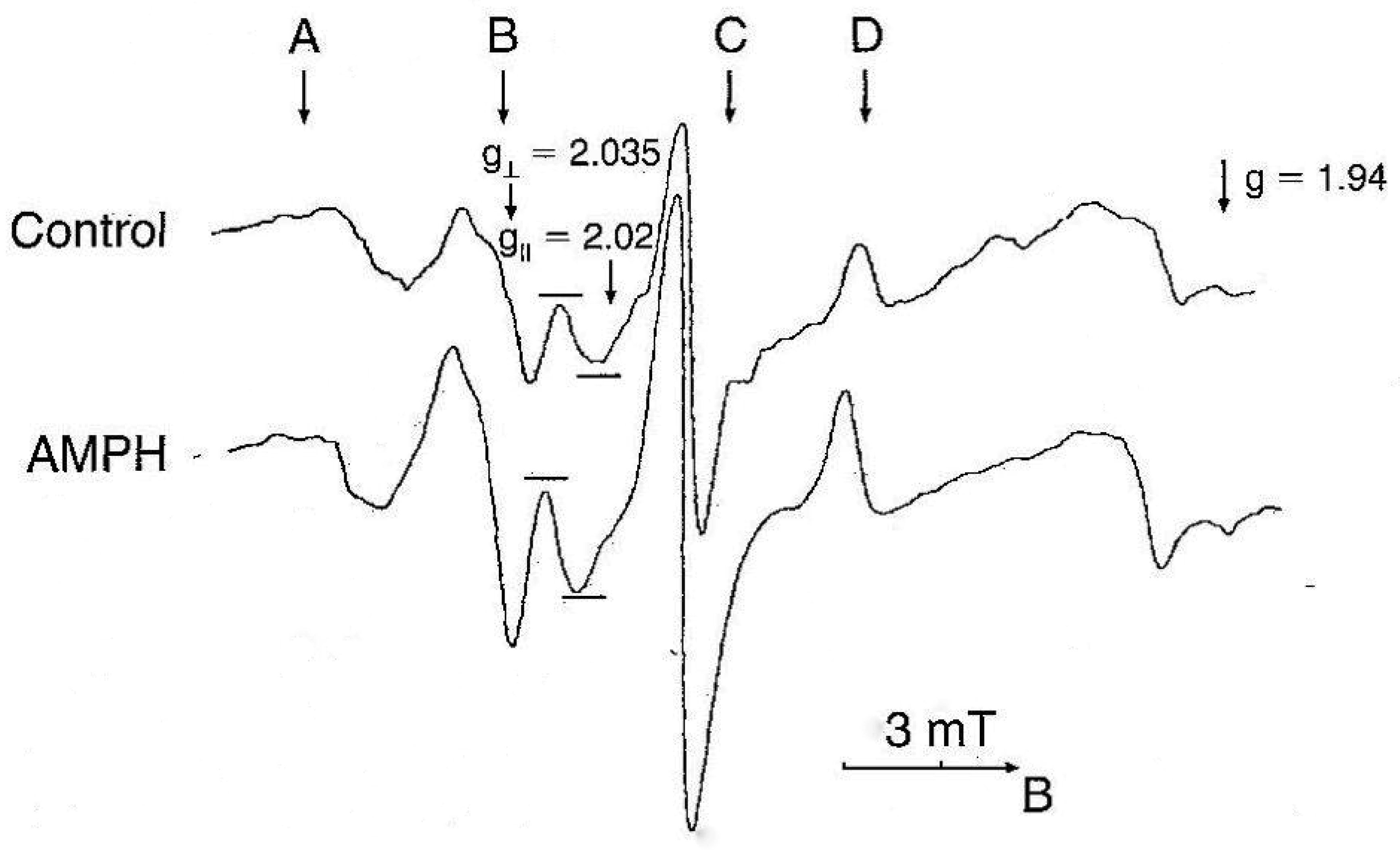
    [44] Bashkatova VG, Mikoian VD, Kosacheva ES, et al. (1996) Direct determination of nitric oxide in rat brain during various types of seizures using ESR. Dokl Akad Nauk 348: 119–121.
    [45] 
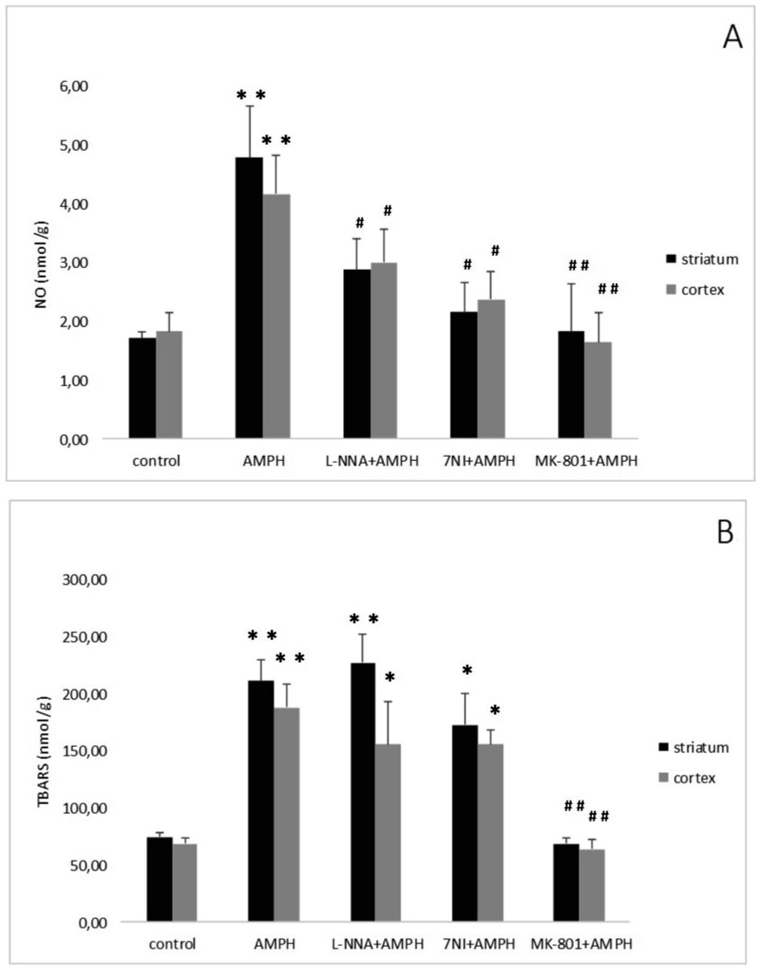
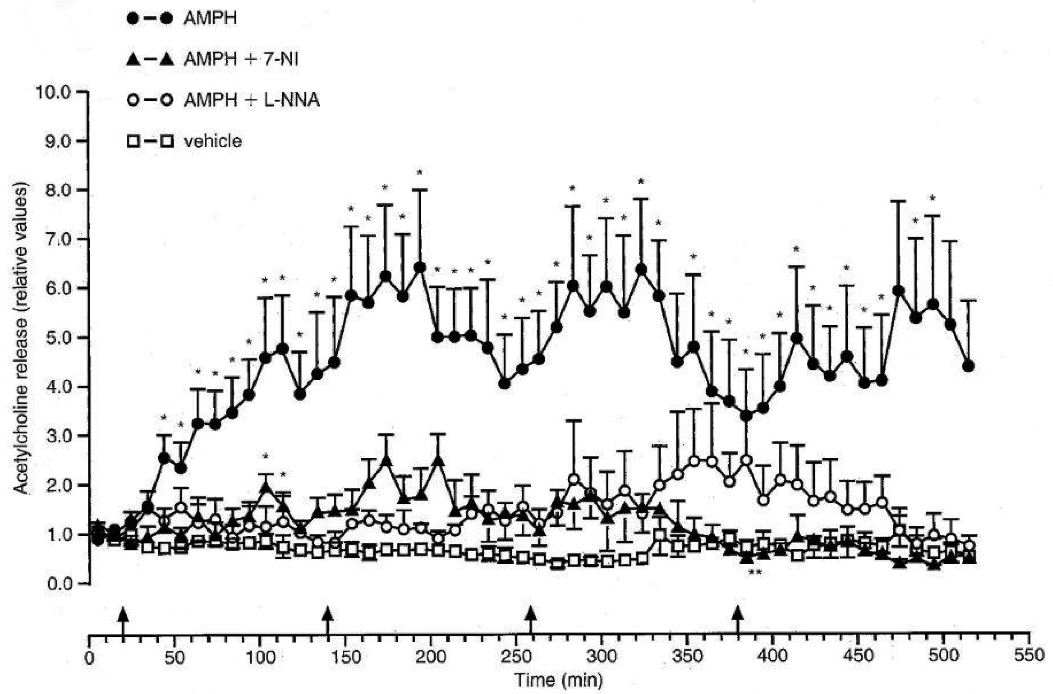
Bashkatova V, Kraus M, Prast H, et al. (1999) Influence of NOS inhibitors on changes in ACH release and NO level in the brain elicited by amphetamine neurotoxicity. Neuroreport 10: 3155–3158. doi: 10.1097/00001756-199910190-00006
    [46] Bashkatova V, Kraus MM, Vanin A, et al. (2005) 7-Nitroindazole, nNOS inhibitor, attenuates amphetamine-induced amino acid release and nitric oxide generation but not lipid peroxidation in the rat brain. J Neural Transm 112: 779–788. doi: 10.1007/s00702-004-0224-x
    [47] 
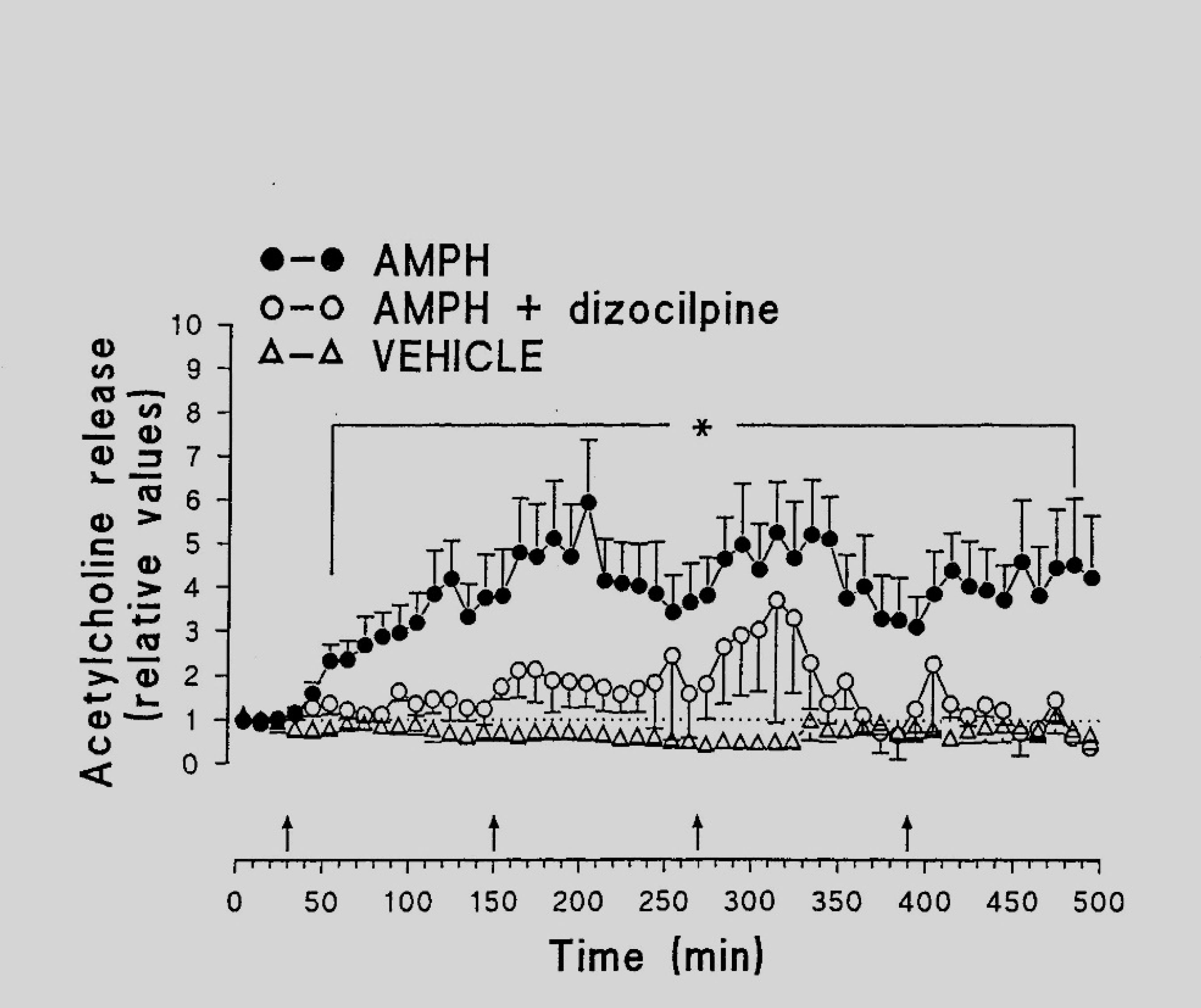
Kraus MM, Bashkatova V, Vanin A, et al. (2002) Dizocilpine inhibits amphetamine-induced formation of nitric oxide and amphetamine-induced release of amino acids and acetylcholine in the rat brain. Neurochem Res 27: 229–235. doi: 10.1023/A:1014836621717
    [48] Wan FJ, Tung CS, Shiah IS, et al. (2006) Effects of alpha-phenyl-N-tert-butyl nitrone and N- acetylcysteine on hydroxyl radical formation and dopamine depletion in the rat striatum produced by d-amphetamine. Eur Neuropsychopharmacol 16: 147–153. doi: 10.1016/j.euroneuro.2005.07.002
    [49] Kita T, Miyazaki I, Asanuma M, et al. (2009) Dopamine-induced behavioral changes and oxidative stress in methamphetamine-induced neurotoxicity. Int Rev Neurobiol 88: 43–64. doi: 10.1016/S0074-7742(09)88003-3
    [50] Dawson TM, Dawson VL, Snyder SH (1994) Molecular mechanisms of nitric oxide actions in the brain. Ann N Y Acad Sci 738: 76–85.
    [51] Li J, Baud O, Vartanian T, et al. (2005) Peroxynitrite generated by inducible nitric oxide synthase and NADPH oxidase mediates microglial toxicity to oligodendrocytes. Proc Natl Acad Sci U S A 102: 9936–9941. doi: 10.1073/pnas.0502552102
    [52] Ali SF, Imam SZ, Itzhak Y (2005) Role of peroxynitrite in methamphetamine-induced dopaminergic neurodegeneration and neuroprotection by antioxidants and selective NOS inhibitors. Ann N Y Acad Sci 1053: 97–98. doi: 10.1196/annals.1344.053
    [53] Ohkawa H, Ohishi N, Yagi K (1979) Assay for lipid peroxides in animal tissues by thiobarbituric acid reaction. Anal Biochem 95: 351–358. doi: 10.1016/0003-2697(79)90738-3
    [54] Bashkatova V, Vitskova G, Narkevich V, et al. (2000) Nitric oxide content measured by ESR-spectroscopy in the rat brain is increased during pentylenetetrazole-induced seizures. J Mol Neurosci 14: 183–190. doi: 10.1385/JMN:14:3:183
    [55] Klyueva YYu, Chepurnov SA, Chepurnova NE, et al. (2001) Role of nitric oxide and lipid peroxidation in mechanisms of febrile convulsions in wistar rat pups. Bull Exp Biol Med 131: 47–49. doi: 10.1023/A:1017530612936
    [56] Prast H, Fischer H, Werner E, et al. (1995) Nitric oxide modulates the release of acetylcholine in the ventral striatum of the freely moving rat. Naunyn-Schmiedebergґs Arch Pharmacol 352: 67–73.
    [57] Issy AC, Dos-Santos-Pereira M, Pedrazzi JFC, et al. (2018) The role of striatum and prefrontal cortex in the prevention of amphetamine-induced schizophrenia-like effects mediated by nitric oxide compounds. Prog Neuropsychopharmacol Biol Psychiatry 86: 353–362. doi: 10.1016/j.pnpbp.2018.03.015
    [58] Salum C, Guimarães FS, Brandão ML, et al. (2006) Dopamine and nitric oxide interaction on the modulation of prepulse inhibition of the acoustic startle response in the Wistar rat. Psychopharmacology (Berl) 185: 133–141. doi: 10.1007/s00213-005-0277-z
    [59] Sonsalla PK, Nicklas WJ, Heikkila RE (1989) Role for excitatory amino acids in methamphetamine-induced nigrostriatal dopaminergic toxicity. Science 243: 398–400. doi: 10.1126/science.2563176
    [60] Tata DA, Yamamoto BK (2007) Interactions between methamphetamine and environmentalstress: role of oxidative stress, glutamate and mitochondrial dysfunction. Addiction 102: 49–60. doi: 10.1111/j.1360-0443.2007.01770.x
    [61] Li MH, Underhill SM, Reed C, et al. (2017) Amphetamine and methamphetamine increaseNMDAR-GluN2B synaptic currents in midbrain dopamine neurons. Neuropsychopharmacology 42: 1539–1547. doi: 10.1038/npp.2016.278
    [62] Haj-Mirzaian A, Amiri S, Amini-Khoei H, et al. (2018) Involvement of NO/NMDA-R pathwayin the behavioral despair induced by amphetamine withdrawal. Brain Res Bull 139: 81–90. doi: 10.1016/j.brainresbull.2018.02.001
    [63] Erenberg G (2005) The relationship between tourette syndrome, attention deficit hyperactivitydisorder, and stimulant medication: a critical review. Semin Pediatr Neurol 12: 217–221. doi: 10.1016/j.spen.2005.12.003
    [64] Jain R, Jain S, Montano CB (2017) Addressing diagnosis and treatment gaps in adults withattention-deficit/hyperactivity disorder. Prim Care Companion CNS Disord 19: pii: 17nr02153.
    [65] Quilty LC, Allen TA, Davis C, et al. (2019) A randomized comparison of long actingmethylphenidate and cognitive behavioral therapy in the treatment of binge eating disorder. Psychiatry Res 273: 467–474. doi: 10.1016/j.psychres.2019.01.066
    [66] Novoselov IA, Cherepov AB, Raevskii KS, et al. (2002) Locomotor activity and expression ofc-Fos protein in the brain of C57BL and Balb/c mice: effects of D-amphetamine and sydnocarb. Eksp Klin Farmakol 65: 18–21.
    [67] Gruner JA, Mathiasen JR, Flood DG, et al. (2011) Characterization of pharmacological andwake-promoting properties of the dopaminergic stimulant sydnocarb in rats. J Pharmacol ExpTher 337: 380–390. doi: 10.1124/jpet.111.178947
    [68] Gainetdinov RR, Sotnikova TD, Grekhova TV, et al. (1997) Effects of a psychostimulant drugsydnocarb on rat brain dopaminergic transmission in vivo. Eur J Pharmacol 340: 53–58. doi: 10.1016/S0014-2999(97)01407-6
    [69] Afanas'ev II, Anderzhanova EA, Kudrin VS, et al. (2001) Effects of amphetamine andsydnocarb on dopamine release and free radical generation in rat striatum. Pharmacol BiochemBehav 200169: 653–658.
    [70] Bashkatova V, Mathieu-Kia AM, Durand C, et al. (2002) Neurochemical changes and neurotoxic effects of an acute treatment with sydnocarb, a novel psychostimulant: comparison with D-amphetamine. Ann N Y Acad Sci 965: 180–192.
    [71] Feier G, Valvassori SS, Lopes-Borges J (2012) Behavioral changes and brain energy metabolism dysfunction in rats treated with methamphetamine or dextroamphetamine. Neurosci Lett 530: 75–79. doi: 10.1016/j.neulet.2012.09.039
    [72] Witkin JM, Savtchenko N, Mashkovsky M, et al. (1999) Behavioral, toxic, and neurochemical effects of sydnocarb, a novel psychomotor stimulant: comparisons with methamphetamine. J Pharmacol Exp Ther 288: 1298–1310.
    [73] Anderzhanova EA, Afanas'ev II, Kudrin VS, et al. (2000) Effect of d-amphetamine and sydnocarb on the extracellular level of dopamine, 3,4-dihydroxyphenylacetic acid, and hydroxyl radicals generation in rat striatum. Ann N Y Acad Sci 914: 137–145. doi: 10.1111/j.1749-6632.2000.tb05191.x
    [74] Chen N, Li J, Li D, et al. (2014) Chronic exposure to perfluorooctane sulfonate induces behavior defects and neurotoxicity through oxidative damages, in vivo and in vitro. PLoS One 9: e113453. doi: 10.1371/journal.pone.0113453
    [75] Zhang LP, Wang QS, Guo X, et al. (2007) Time-dependent changes of lipid peroxidation and antioxidative status in nerve tissues of hens treated with tri-ortho-cresyl phosphate (TOCP). Toxicology 239: 45–52. doi: 10.1016/j.tox.2007.06.091
  • Reader Comments
  • © 2019 the Author(s), licensee AIMS Press. This is an open access article distributed under the terms of the Creative Commons Attribution License (http://creativecommons.org/licenses/by/4.0)
通讯作者: 陈斌, bchen63@163.com
  • 1. 

    沈阳化工大学材料科学与工程学院 沈阳 110142

  1. 本站搜索
  2. 百度学术搜索
  3. 万方数据库搜索
  4. CNKI搜索

Metrics

Article views(6616) PDF downloads(640) Cited by(6)

Other Articles By Authors

/

DownLoad:  Full-Size Img  PowerPoint
Return
Return

Catalog