Evaluating public expenditures on tourism: the utility of the Italian public accounting reforms

Fabrizio Antolini; Fabrizio Antolini

doi:10.3934/NAR.2021009

National Accounting Review

2021, Volume 3, Issue 2: 179-203. doi: 10.3934/NAR.2021009

Previous Article Next Article

Research article Special Issues

Evaluating public expenditures on tourism: the utility of the Italian public accounting reforms

Fabrizio Antolini ^,

University of Teramo, CAMPUS Universitario "A. Saliceti", Contrada, Coste Sant'Agostino, Via Renato Balzarini, 1, 64100 Teramo, Italy

Received: 13 January 2021 Accepted: 13 April 2021 Published: 20 April 2021
JEL Codes: H10, H50, H61, H72, M38, M41, P24, P41

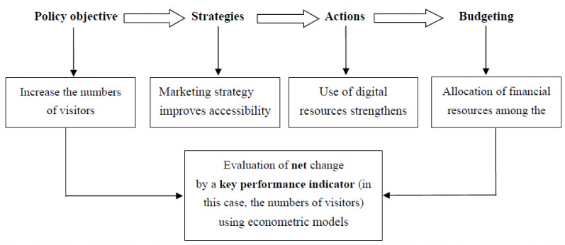
The accounting reforms of the state, regional and local budgets that began in 2009 and finished in 2016 have improved the quality of public accounting data. Mainly, these reforms were completed for the adoption of the functional classification of expenditures in the administrative balances of all Public Administration (PA) entities. This process is the same one that is utilized in government financial statistics for the Macroeconomic Imbalance Procedure (MIP), even if some differences remain. However, to evaluate the effectiveness of political actions it is necessary, first of all, to have a reference scheme, identifying a recognized set of Key Performance Indicators (KPIs). Public expenditure after the public accounting reform, is linked to the policies undertaken and this is particularly useful to assess it. As far as tourism is concerned, in order to have an adequate measure of the resources managed in tourism field, it is necessary to consider as public domain the Enlarged Public Sector (EPS), including also public enterprise. Using arrivals and nights spent as KPIs in a panel econometric model, this research examines the net change over time. In the model, the explicative variables are "public tourism expenditures" and "environment, transport and mobility expenditures" considering the EPS sector as referred domains in the period 2000–2017.
- national account,
- Italian accounting reform,
- public tourism expenditures,
- evaluation,
- panel econometric model
Citation: Fabrizio Antolini. Evaluating public expenditures on tourism: the utility of the Italian public accounting reforms[J]. National Accounting Review, 2021, 3(2): 179-203. doi: 10.3934/NAR.2021009

Related Papers:

Abstract

The accounting reforms of the state, regional and local budgets that began in 2009 and finished in 2016 have improved the quality of public accounting data. Mainly, these reforms were completed for the adoption of the functional classification of expenditures in the administrative balances of all Public Administration (PA) entities. This process is the same one that is utilized in government financial statistics for the Macroeconomic Imbalance Procedure (MIP), even if some differences remain. However, to evaluate the effectiveness of political actions it is necessary, first of all, to have a reference scheme, identifying a recognized set of Key Performance Indicators (KPIs). Public expenditure after the public accounting reform, is linked to the policies undertaken and this is particularly useful to assess it. As far as tourism is concerned, in order to have an adequate measure of the resources managed in tourism field, it is necessary to consider as public domain the Enlarged Public Sector (EPS), including also public enterprise. Using arrivals and nights spent as KPIs in a panel econometric model, this research examines the net change over time. In the model, the explicative variables are "public tourism expenditures" and "environment, transport and mobility expenditures" considering the EPS sector as referred domains in the period 2000–2017.

References

[1]	Antolini F, Truglia FG (2019) Ecotourism and food geographical areas, In: Carpita-Fabbris, M. Carpita, L. Fabbris, Asa Conference, Statistics for Health and Well-being Book of Short Paper. Isbn: 9788854951358
[2]	Antolini F, Giusti A, Grassini L (2017) Attrattività dei territori e flussi turistici: l'importanza di una corretta programmazione settoriale. Turistica, 1–31.
[3]	Antolini F, Grassini L (2019) Il turismo nella statistica ufficiale, Convegno sul turismo sensoriale, Florence University.
[4]	Arellano M (1987) Computing Robust Standard Errors for within Group Estimators. Oxf Bull Econ Stat 49: 431–434.
[5]	Arellano M (2003) Panel Data Econometrics, Oxford University Press.
[6]	Aschauer DA (1989) Is public expenditure productive? J Monetary Econ 23: 177–200. doi: 10.1016/0304-3932(89)90047-0
[7]	Baltagi BH, Li Q (1995) Testing AR (1) against MA (1) disturbances in an error component model. J Econometrics 68: 133–151. doi: 10.1016/0304-4076(94)01646-H
[8]	Baltagi B (2008) Econometric analysis of panel data, John Wiley & Sons.
[9]	Barnes M, Matka E, Sullivan H (2003) Evidence, understanding and complexity: evaluation in non-linear systems. Evaluation 9: 265–284. doi: 10.1177/13563890030093003
[10]	Birkland TA (2019) An introduction to the policy process: Theories, concepts, and models of public policy making, Routledge.
[11]	Chan JL (2010) IPSAS: Conceptual and Institutional Issues. Chan GA Seminar, 1–96.
[12]	Chuaire MF, Scartascini C, Tommasi M (2017) State capacity and the quality of policies. Revisiting the relationship between openness and government size. Econ Policies 29: 133–156.
[13]	Clements MP, Joutz F, Stekler HO (2007) An evaluation of the forecasts of the Federal Reserve: a pooled approach. J Appl Econometrics 22: 121–136. doi: 10.1002/jae.954
[14]	Cooper RN (1985) Economic interdependence and coordination of economic policies. Handb Int Econ 2: 1195–1234. doi: 10.1016/S1573-4404(85)02014-7
[15]	Commissione Parlamentare per le Questioni Regionali (2016) Resoconto stenografico, Seduta n. 23 di Giovedì 13 ottobre 2016, Roma.
[16]	Cuccu O, De Luca S (2006) The Policies and the planning instruments for Tourism, In: Svimez, Report on Tourism Industry in the Mezzogiorno, Il Mulino, Bologna.
[17]	Dabbicco G (2015) The impact of accrual-based public accounting harmonization on EU macroeconomic surveillance and governments' policy decision-making. Int J Public Adm 38: 253–267. doi: 10.1080/01900692.2015.999581
[18]	Dasí RM, Montesinos V, Murgui S (2016) Government financial statistics and accounting in Europe: is ESA 2010 improving convergence? Public Money Manage 36: 165–172. doi: 10.1080/09540962.2016.1133964
[19]	De Jesus MAJ, Jorge SM (2011) Cash-accruals adjustments from governmental accounting to national accounts: Implications on the Italian, Portuguese and Spanish central governmental budgetary balances, In: XVI Congreso AECA-Nuevo modelo económico: Empresa, Mercados y Culturas.
[20]	Devarajan S, Swaroop V, Zou HF (1996) The composition of public expenditure and economic growth. J Monetary Econ 37: 313–344. doi: 10.1016/0304-3932(96)01249-4
[21]	Dwyer L, Forsyth P, Spurr R (2007) Contrasting the Uses of TSAs and CGE models: Measuring Tourism Yield and Productivity. Tourism Econ 13: 537–551. doi: 10.5367/000000007782696096
[22]	Eurostat (1996) European System of Accounts (ESA). Luxembourg.
[23]	Eurostat (2010) European System of Accounts (ESA). Luxemburg.
[24]	Eurostat (2014), Methodological manual for tourism statistics, version 3.1. Available from https://ec.europa.eu/eurostat/documents/3859598/6454997/KS-GQ-14-013-EN-N.pdf/166605aa-c990-40c4-b9f7-59c297154277?t=1420557603000.
[25]	Gerrard CD, Ferroni M, Mody A (2001) Global Public Policies and Programs: Implications for Financing and Evaluation. The World Bank.
[26]	Giungato G, Tancredi A (2019) Confronto tra il sistema CPT e i Conti delle Amministrazioni Pubbliche Istat. In: CPT Informa.
[27]	Grassini L, Dugheri G (2021) Mobile phone data and tourism statistics: a broken promise? Natl Accounting Rev 3: 50–68. doi: 10.3934/NAR.2021002
[28]	Haynes P (2008) Complexity theory and evaluation in public management: A qualitative systems approach. Public Manage Rev 10: 401–419. doi: 10.1080/14719030802002766
[29]	Howlett M (2019) Designing public policies: Principles and instruments, Routledge.
[30]	Innes JE, Booher DE (2018) Planning with complexity: An introduction to collaborative rationality for public policy, Routledge.
[31]	Istat (2000) Movimento negli Esercizi Ricettivi, Roma.
[32]	Key VO (1940) The lack of a budgetary theory. Am Political Sci Rev 34: 1137–1144. doi: 10.2307/1948194
[33]	Leruth MLE, Paul E (2006) A principal-agent theory approach to public expenditure management systems in developing countries. IMF Working Paper No. 06/204.
[34]	Mahadi R, Khalid SNA, Mail R, et al. (2017) Accrual Accounting in Public Sectors: Possible Contextual and Application Gaps for Future Research Agenda. Asian J Financ Accounting 9.
[35]	Monteiro BRP, Gomes RC (2013) International experiences with accrual budgeting in the public sector. Revista Contabilidade Finanças 24: 103.
[36]	OECD (2004) Evaluation of Sme policies and programmes. Promoting Entrepreneurship and Innovative SMEs in a Global Economy: Towards a more responsible and inclusive Globalization. Istanbul Turkey.
[37]	Oxman AD, Bjørnda, A, Becerra-Posada F, et al. (2010) A framework for mandatory impact evaluation to ensure well informed public policy decisions. Lancet 375: 427–431. doi: 10.1016/S0140-6736(09)61251-4
[38]	Peter Van der Hoek M (2005) From cash to accrual budgeting and accounting in the public sector: The Dutch experience. Public Budg Financ 25: 32–45. doi: 10.1111/j.0275-1100.2005.00353.x
[39]	Pollack M (1995) Regional Actors in an intergovernmental play: the making and implementation of EC structural policy, In: Rhodes C and Mazey S, The state of the European Union, (eds.), Longman: Harlow.
[40]	Scriven M (1991) Evaluation thesaurus, 4th Edition, Sage, Newbury Park.
[41]	Setiyawati H, Iskandar D, Basar YS (2018) The quality of financial reporting through increasing the competence of internal accountants and accrual basis. Int J Econ Bus Manage Stud 5: 31–40. doi: 10.20448/802.51.31.39
[42]	Storey D (2004) Evaluation of SME Policies and Programmes, presented at 2nd Conference of Ministers Responsible for Small and Medium Sized Enterprises, OECD, Paris (online), available from: http://www.oecd.org/cfe/smes/31919294.pdf.
[43]	Tran VH, Jo V, Pham QT (2020) Vietnam's sustainable tourism and growth: a new approach to strategic policy modelling. Natl Accounting Rev 2: 324–336. doi: 10.3934/NAR.2020019
[44]	United Nations (1999) Classifications of expenditure according to purpose: COFOG, COICOP, COPNI, COPP. In: Series M, Miscellaneous Statistical, Papers, No. 84, New York. Available from: https://unstats.un.org/unsd/classifications/Family/Detail/4.
[45]	United Nations (2008) System of National Accounts, (SNA), Washington.
[46]	Wooldridge J (2001) Econometric Analysis of Cross Section and Panel Data, Cambridge.
[47]	Zeynep O (2000) Determinants of health outcomes in industrialized countries: a pooled, cross- countries, time series analysis OECD. Econ Stud 30: 53–78.

Reader Comments

Your name:*

Email:*
© 2021 the Author(s), licensee AIMS Press. This is an open access article distributed under the terms of the Creative Commons Attribution License (http://creativecommons.org/licenses/by/4.0)